The `DeeDeeExperiment` User's Guide
Najla Abassi
Institute of Medical Biostatistics, Epidemiology and Informatics (IMBEI), Mainzabassina@uni-mainz.de
Lea Schwarz
Institute of Medical Biostatistics, Epidemiology and Informatics (IMBEI), Mainzlea.schwarz@uni-mainz.de
Federico Marini
Institute of Medical Biostatistics, Epidemiology and Informatics (IMBEI), MainzResearch Center for Immunotherapy (FZI), Mainzmarinif@uni-mainz.de
19 May 2026
Source:vignettes/DeeDeeExperiment_manual.Rmd
DeeDeeExperiment_manual.RmdIntroduction
Why do we need a new class?
Differential expression analysis (DEA) and functional enrichment analysis (FEA) are core steps in transcriptomic workflows, helping researchers detect and interpret biological differences between conditions. However, as the number of conditions (defined by complex experimental designs) and analysis tools increases, managing the outputs of these analyses across multiple contrasts becomes increasingly overwhelming. This challenge is further amplified in single-cell RNA-seq, where pseudo-bulk analyses generate numerous results tables across cell types and contrasts, making it challenging to organize, explore, and reproduce findings, even for experienced users - we invite you to see this more in detail in the dedicated companion vignette for single cell data.
To address these issues, we introduce the DeeDeeExperiment
class, an S4 object that extends the widely adopted
SingleCellExperiment class in Bioconductor.
DeeDeeExperiment provides a structured and consistent
framework for integrating DEA and FEA results alongside core expression
data and metadata. By centralizing these results in a single container,
DeeDeeExperiment enables users to retrieve, explore, and
manage their analysis results more efficiently across multiple
contrasts.
This vignette introduces the class structure, demonstrates how to
create and work with DeeDeeExperiment objects, and walks
through a typical RNA-seq workflow using the class.
Anatomy of DeeDeeExperiment
The DeeDeeExperiment class inherits from the core
Bioconductor SingleCellExperiment object. This means it
inherits all the slots, methods, and compatibility with tools built for
SingleCellExperiment, while introducing additional
components to streamline downstream analysis.
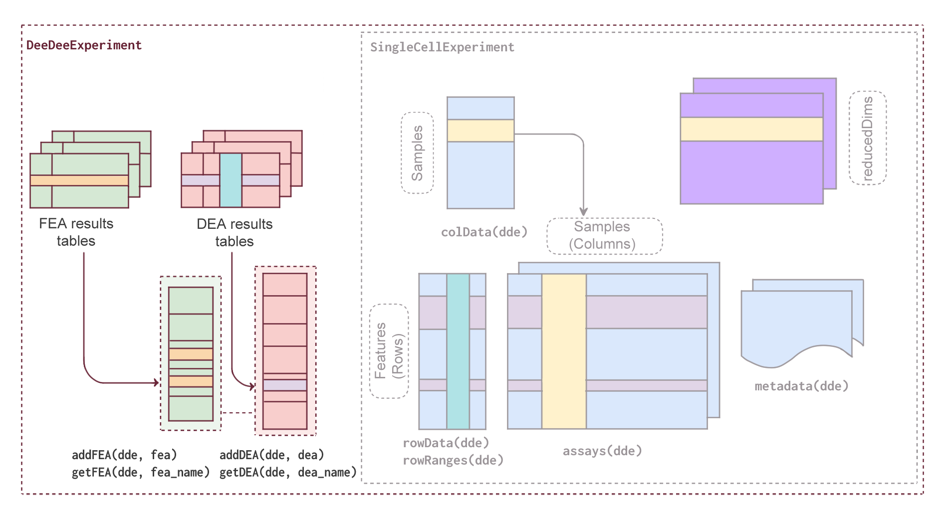
Specifically, DeeDeeExperiment has two new slots:
-
dea: aSimpleListthat stores results from differential expression analysis (DEA), along with relevant metadata. This includes:- The used False Discovery Rate (FDR) and log2 fold change (LFC) thresholds (if specified).
- Meta info related to both the LFC and p-value.
- The package used to generate the DE results (e.g. DEseq2, edgeR or limma…).
- A pointer to the original DE result object, which is kept in the
metadataof theDeeDeeExperimentobject.
The main columns to use in DEA in addition to the feature identifier
(log2FoldChange, pvalue, and
padj) are also stored in the rowData of the
DeeDeeExperiment object.
-
fea: aSimpleListthat stores results from functional enrichment analysis (FEA), along with relevant metadata. This includes:- The name of the associated DEA contrast.
- The FEA name.
- A
GeneTonicList-compatible set ofshaken_results(ready to be used in GeneTonic). - The enrichment tool used to generate the results
(e.g.
topGO,clusterProfiler...). - A copy of the original enrichment result object.
The SimpleList slot type will bring the advantage of
storing DEA/FEA related metadata (e.g., the design formula) directly
into its metadata/mcols.
Creating a DeeDeeExperiment object
In order to create a DeeDeeExperiment object, at least
one of the following inputs are required:
-
sce: ASingleCellExperimentobject, that will be used as a scaffold to store the DE related information. -
de_results: A named list of DE results, in any of the formats supported by the package (currently results fromDESeq2,edgeR,limma, ormuscat). -
enrich_results: A named list of FE results, asdata.framegenerated by one of the following packages (currentlytopGO,clusterProfiler,enrichR,gProfiler,fgsea,gsea,DAVID, and output ofGeneTonicshakers)
# do not run
dde <- DeeDeeExperiment(
  sce = sce, # sce is a SingleCellExperiment object
  # de_results is a named list of de results
  de_results = de_results,
  # enrich_res is a named list of enrichment results
  enrich_results = enrich_results
)
Getting started
To install this package, start R and enter:
if (!requireNamespace("BiocManager", quietly = TRUE)) {
  install.packages("BiocManager")
}

BiocManager::install("DeeDeeExperiment")
Once installed, the package can be loaded and attached to your current workspace as follows:
DeeDeeExperiment on the macrophage
dataset
In the remainder of this vignette, we will illustrate the main features of DeeDeeExperiment on a publicly available dataset from Alasoo, et al. “Shared genetic effects on chromatin and gene expression indicate a role for enhancer priming in immune response”, published in Nature Genetics, January 2018 (Alasoo et al. 2018) doi:10.1038/s41588-018-0046-7.
The data is made available via the macrophage Bioconductor package, which contains the files output from the Salmon quantification (version 0.12.0, with GENCODE v29 reference), as well as the values summarized at the gene level, which we will use to exemplify.
In the macrophage experimental setting, the samples are
available from 6 different donors, in 4 different conditions (naive,
treated with Interferon gamma, with SL1344, or with a combination of
Interferon gamma and SL1344).
Let’s start by loading all the necessary packages:
library("DeeDeeExperiment")

library("macrophage")
library("DESeq2")
library("edgeR")
library("DEFormats")
We will demonstrate how DeeDeeExperiment fits into a
regular bulk RNA-seq data analysis workflow. For this we will start by
processing the data and setting up the design for the Differential
Expression Analysis (DEA).
# load data
data(gse, package = "macrophage")
If you already have your differential expression results and want to
skip the DEA workflow examples, you can jump directly to the section 4 Creating
DeeDeeExperiment the DeeDee way - otherwise, you can follow along in
the subsequent sections where we will showcase how the typical objects
from each DE framework will seamlessly fit into a
DeeDeeExperiment object.
The remainder of this vignette assumes some knowledge of Differential
Expression Analysis workflows. If you want some excellent introductions
to this topic, you can refer to (Love et al.
2016) and (Law et al. 2018) -
Otherwise, you can check (Ludt et al.
2022) for a comprehensive overview of these workflows, as well as
the usage of tools such as GeneTonic or
pcaExproler for interactive exploration.
DEA: DESeq2 framework
Below we will demonstrate an example on how to generate DE results
with DESeq2
# set up design
dds_macrophage <- DESeqDataSet(gse, design = ~ line + condition)
rownames(dds_macrophage) <- substr(rownames(dds_macrophage), 1, 15)
keep <- rowSums(counts(dds_macrophage) >= 10) >= 6

dds_macrophage <- dds_macrophage[keep, ]
For the sake of demonstration, we will further subset the dataset for faster processing
# set seed for reproducibility
set.seed(42)
# sample randomly for 1k genes to speed up the processing
selected_genes <- sample(rownames(dds_macrophage), 1000)

dds_macrophage <- dds_macrophage[selected_genes, ]
We then run the main DESeq() function and check the
resultsNames being generated
dds_macrophage
#> class: DESeqDataSet
#> dim: 1000 24
#> metadata(7): tximetaInfo quantInfo ... txdbInfo version
#> assays(3): counts abundance avgTxLength
#> rownames(1000): ENSG00000164741 ENSG00000078808 ... ENSG00000273680
#>   ENSG00000073536
#> rowData names(2): gene_id SYMBOL
#> colnames(24): SAMEA103885102 SAMEA103885347 ... SAMEA103885308
#>   SAMEA103884949
#> colData names(15): names sample_id ... condition line
# run DESeq
dds_macrophage <- DESeq(dds_macrophage)
# contrasts
resultsNames(dds_macrophage)
#> [1] "Intercept"                      "line_eiwy_1_vs_diku_1"
#> [3] "line_fikt_3_vs_diku_1"          "line_ieki_2_vs_diku_1"
#> [5] "line_podx_1_vs_diku_1"          "line_qaqx_1_vs_diku_1"
#> [7] "condition_IFNg_vs_naive"        "condition_IFNg_SL1344_vs_naive"
#> [9] "condition_SL1344_vs_naive"
Let’s extract the DE results for each contrast. We will only use two contrasts
FDR <- 0.05
# IFNg_vs_naive
IFNg_vs_naive <- results(dds_macrophage,
                         name = "condition_IFNg_vs_naive",
                         lfcThreshold = 1,
                         alpha = FDR
)
IFNg_vs_naive <- lfcShrink(dds_macrophage,
                           coef = "condition_IFNg_vs_naive",
                           res = IFNg_vs_naive,
                           type = "apeglm"
)

# Salm_vs_naive
Salm_vs_naive <- results(dds_macrophage,
                         name = "condition_SL1344_vs_naive",
                         lfcThreshold = 1,
                         alpha = FDR
)
Salm_vs_naive <- lfcShrink(dds_macrophage,
                           coef = "condition_SL1344_vs_naive",
                           res = Salm_vs_naive,
                           type = "apeglm"
)

head(IFNg_vs_naive)
#> log2 fold change (MAP): condition IFNg vs naive
#> Wald test p-value: condition IFNg vs naive
#> DataFrame with 6 rows and 5 columns
#>                  baseMean log2FoldChange     lfcSE      pvalue        padj
#>                 <numeric>      <numeric> <numeric>   <numeric>   <numeric>
#> ENSG00000164741  918.0347      0.2291487 0.3006751 9.80541e-01 1.00000e+00
#> ENSG00000078808 6684.4755     -0.0115336 0.0729923 1.00000e+00 1.00000e+00
#> ENSG00000251034   12.1241     -0.1167013 0.4049828 9.33899e-01 1.00000e+00
#> ENSG00000162676   10.2220      0.2691481 0.3776971 9.00817e-01 1.00000e+00
#> ENSG00000170356   15.0772     -0.1278637 0.3522078 9.72815e-01 1.00000e+00
#> ENSG00000204257 1922.0256      4.0550244 0.1960055 1.67298e-56 8.36488e-54
head(Salm_vs_naive)
#> log2 fold change (MAP): condition SL1344 vs naive
#> Wald test p-value: condition SL1344 vs naive
#> DataFrame with 6 rows and 5 columns
#>                  baseMean log2FoldChange     lfcSE    pvalue      padj
#>                 <numeric>      <numeric> <numeric> <numeric> <numeric>
#> ENSG00000164741  918.0347      0.0114691 0.3224207  0.999632  1.000000
#> ENSG00000078808 6684.4755      0.7893601 0.0734122  0.997559  1.000000
#> ENSG00000251034   12.1241      1.1881497 0.4894973  0.226918  0.982042
#> ENSG00000162676   10.2220      0.4420821 0.4228376  0.843212  1.000000
#> ENSG00000170356   15.0772     -0.6249201 0.4252786  0.726972  1.000000
#> ENSG00000204257 1922.0256     -0.7293810 0.2005145  0.883888  1.000000
We now have two DESeqResults objects:
IFNg_vs_naive and Salm_vs_naive, ready to be
integrated into a DeeDeeExperiment object.
DEA: limma framework
Not working with DESeq2? No problem.
DeeDeeExperiment is method-agnostic and easily integrates
results from other frameworks like limma. In this section,
we will walk through a typical limma workflow to generate
DE results.
For demonstration purposes, we convert the filtered
dds_macrophage as input for limma, using the
as.DGEList() function from the DEFormats
package.
# create DGE list
dge <- DEFormats::as.DGEList(dds_macrophage)
We then normalize and voom-transform the expression values, before
running the lmFit() function:
# normalize the counts
dge <- calcNormFactors(dge)

# create design for DE
design <- model.matrix(~ line + group, data = dge$samples)
# transform counts into logCPM
v <- voom(dge, design)

# fitting linear models using weighted least squares for each gene
fit <- lmFit(v, design)
We define here as usual the contrast matrix:
# available comparisons
colnames(design)
#> [1] "(Intercept)"      "lineeiwy_1"       "linefikt_3"       "lineieki_2"
#> [5] "linepodx_1"       "lineqaqx_1"       "groupIFNg"        "groupIFNg_SL1344"
#> [9] "groupSL1344"
# setup comparisons
contrast_matrix <- makeContrasts(
  IFNg_vs_Naive = groupIFNg,
  Salm_vs_Naive = groupSL1344,
  levels = design
)
We then extract the results by applying the
contrasts.fit function, followed by the empirical Bayes
moderation as it follows:
# apply contrast
fit2 <- contrasts.fit(fit, contrast_matrix)

# empirical Bayes moderation of standard errors
fit2 <- eBayes(fit2)
de_limma <- fit2 # MArrayLM object
We show here the top 10 DE genes, as detected in the contrast
IFNg_vs_Naive
# show top 10 genes, first columns
topTable(de_limma, coef = "IFNg_vs_Naive", number = 10)[, 1:7]
#>                 seqnames     start       end  width strand            gene_id
#> ENSG00000204257     chr6  32948613  32969094  20482      - ENSG00000204257.14
#> ENSG00000231389     chr6  33064569  33080775  16207      -  ENSG00000231389.7
#> ENSG00000123992     chr2 219373527 219400022  26496      - ENSG00000123992.19
#> ENSG00000227531     chr9 111139246 111284836 145591      -  ENSG00000227531.1
#> ENSG00000197448     chr7 143244093 143270854  26762      + ENSG00000197448.13
#> ENSG00000100418    chr22  41598028  41621096  23069      -  ENSG00000100418.7
#> ENSG00000065911     chr2  74198562  74217565  19004      + ENSG00000065911.11
#> ENSG00000233621     chr1  37454879  37474411  19533      -  ENSG00000233621.1
#> ENSG00000143771     chr1 224356850 224379459  22610      + ENSG00000143771.11
#> ENSG00000135124    chr12 121209857 121234106  24250      + ENSG00000135124.14
#>                    SYMBOL
#> ENSG00000204257   HLA-DMA
#> ENSG00000231389  HLA-DPA1
#> ENSG00000123992     DNPEP
#> ENSG00000227531      <NA>
#> ENSG00000197448     GSTK1
#> ENSG00000100418     DESI1
#> ENSG00000065911    MTHFD2
#> ENSG00000233621 LINC01137
#> ENSG00000143771     CNIH4
#> ENSG00000135124     P2RX4
We now have a MArrayLM object: de_limma,
ready to be integrated into a DeeDeeExperiment object.
DEA: edgeR framework
Below we will walk you through a typical edgeR pipeline
to produce DE results ready for integration in
DeeDeeExperiment.
We reuse the normalized DGEList and design matrix from
the previous limma workflow (again, created via
DEFormats::as.DGEList()):
dge <- DEFormats::as.DGEList(dds_macrophage)

# estimate dispersion
dge <- estimateDisp(dge, design)
# perform likelihood ratio test
fit <- glmFit(dge, design)
Here as well, we define the contrasts of interest:
# available comparisons
colnames(design)
#> [1] "(Intercept)"      "lineeiwy_1"       "linefikt_3"       "lineieki_2"
#> [5] "linepodx_1"       "lineqaqx_1"       "groupIFNg"        "groupIFNg_SL1344"
#> [9] "groupSL1344"
# setup comparisons
contrast_matrix <- makeContrasts(
  IFNg_vs_Naive = groupIFNg,
  Salm_vs_Naive = groupSL1344,
  levels = design
)
… and. we create the DGELRT objects to store the DE
results as follows:
# DGELRT objects
dge_lrt_IFNg_vs_naive <- glmLRT(fit,
                                contrast = contrast_matrix[, "IFNg_vs_Naive"])
dge_lrt_Salm_vs_naive <- glmLRT(fit,
                                contrast = contrast_matrix[, "Salm_vs_Naive"])
The top 10 DE genes computed within the edgeR framework can be shown as in this chunk:
# show top 10 genes, first few columns
topTags(dge_lrt_IFNg_vs_naive, n = 10)[, 1:7]
#> Coefficient:  1*groupIFNg
#>                 seqnames     start       end  width strand            gene_id
#> ENSG00000204257     chr6  32948613  32969094  20482      - ENSG00000204257.14
#> ENSG00000231389     chr6  33064569  33080775  16207      -  ENSG00000231389.7
#> ENSG00000123992     chr2 219373527 219400022  26496      - ENSG00000123992.19
#> ENSG00000227531     chr9 111139246 111284836 145591      -  ENSG00000227531.1
#> ENSG00000197448     chr7 143244093 143270854  26762      + ENSG00000197448.13
#> ENSG00000233621     chr1  37454879  37474411  19533      -  ENSG00000233621.1
#> ENSG00000065911     chr2  74198562  74217565  19004      + ENSG00000065911.11
#> ENSG00000135124    chr12 121209857 121234106  24250      + ENSG00000135124.14
#> ENSG00000163131     chr1 150730196 150765957  35762      - ENSG00000163131.10
#> ENSG00000100418    chr22  41598028  41621096  23069      -  ENSG00000100418.7
#>                    SYMBOL
#> ENSG00000204257   HLA-DMA
#> ENSG00000231389  HLA-DPA1
#> ENSG00000123992     DNPEP
#> ENSG00000227531      <NA>
#> ENSG00000197448     GSTK1
#> ENSG00000233621 LINC01137
#> ENSG00000065911    MTHFD2
#> ENSG00000135124     P2RX4
#> ENSG00000163131      CTSS
#> ENSG00000100418     DESI1
For the sake of demonstrating that DeeDeeExperiment can
handle the different objects from the edgeR framework, we
also compute some results with the exactTest()
approach.
# perform exact test
# exact test doesn't handle multi factor models, so we have to subset

# IFNg vs naive
keep_samples <- dge$samples$group %in% c("naive", "IFNg")
dge_sub <- dge[, keep_samples]
# droplevel
group <- droplevels(dge_sub$samples$group)
dge_sub$samples$group <- group

# recalculate normalization and dispersion
dge_sub <- calcNormFactors(dge_sub)
dge_sub <- estimateDisp(dge_sub, design = model.matrix(~group))
# exact test
# DGEExact object
dge_exact_IFNg_vs_naive <- exactTest(dge_sub, pair = c("naive", "IFNg"))


# SL1344 vs naive
keep_samples <- dge$samples$group %in% c("naive", "SL1344")
dge_sub <- dge[, keep_samples]
# droplevel
group <- droplevels(dge_sub$samples$group)
dge_sub$samples$group <- group

# recalculate normalization and dispersion
dge_sub <- calcNormFactors(dge_sub)
dge_sub <- estimateDisp(dge_sub, design = model.matrix(~group))
# exact test
dge_exact_Salm_vs_naive <- exactTest(dge_sub, pair = c("naive", "SL1344"))
Again, the top 10 DE genes in the
dge_exact_Salm_vs_naive object can be shown with
topTags(dge_exact_Salm_vs_naive, n = 10)[, 1:7]
#> Comparison of groups:  SL1344-naive
#>                 seqnames     start       end  width strand            gene_id
#> ENSG00000234394     chr9  68306528  68330626  24099      +  ENSG00000234394.8
#> ENSG00000132405     chr4   6909242   7033118 123877      + ENSG00000132405.18
#> ENSG00000109756     chr4 159103013 159360174 257162      +  ENSG00000109756.9
#> ENSG00000078804    chr20  34704290  34713439   9150      + ENSG00000078804.12
#> ENSG00000105711    chr19  35030466  35040449   9984      + ENSG00000105711.11
#> ENSG00000188211    chr11  17351726  17377341  25616      +  ENSG00000188211.8
#> ENSG00000214113     chr6   5102593   5260939 158347      - ENSG00000214113.10
#> ENSG00000253535     chr8  24295814  24912073 616260      -  ENSG00000253535.5
#> ENSG00000179826    chr11  18120955  18138480  17526      +  ENSG00000179826.6
#> ENSG00000183246    chr22  21545357  21551461   6105      -  ENSG00000183246.6
#>                   SYMBOL
#> ENSG00000234394     <NA>
#> ENSG00000132405  TBC1D14
#> ENSG00000109756  RAPGEF2
#> ENSG00000078804 TP53INP2
#> ENSG00000105711    SCN1B
#> ENSG00000188211  NCR3LG1
#> ENSG00000214113    LYRM4
#> ENSG00000253535     <NA>
#> ENSG00000179826  MRGPRX3
#> ENSG00000183246  RIMBP3C
We now have two DGELRT & two DGEExact
objects: dge_lrt_IFNg_vs_naive,
dge_lrt_Salm_vs_naive &
dge_exact_IFNg_vs_naive,
dge_exact_Salm_vs_naive respectively, ready to be
integrated into a DeeDeeExperiment object.
For demonstration purposes, we will use precomputed FEA results
generated with run_topGO() (a practical wrapper provided by
the mosdef package), and with the gost()
function from gprofiler2 package.
# load Functional Enrichment Analysis results examples
data("topGO_results_list", package = "DeeDeeExperiment")
data("gost_res", package = "DeeDeeExperiment")
data("clusterPro_res", package = "DeeDeeExperiment")
The enrichment results can be displayed in a summary way with these commands:
# ifng vs naive
head(topGO_results_list$ifng_vs_naive)
#>        GO.ID
#> 1 GO:0002822
#> 2 GO:0002697
#> 3 GO:0002250
#> 4 GO:1904064
#> 5 GO:0042098
#> 6 GO:0070663
#>                                                                                                                                      Term
#> 1 regulation of adaptive immune response based on somatic recombination of immune receptors built from immunoglobulin superfamily domains
#> 2                                                                                                   regulation of immune effector process
#> 3                                                                                                                adaptive immune response
#> 4                                                                                   positive regulation of cation transmembrane transport
#> 5                                                                                                                    T cell proliferation
#> 6                                                                                                   regulation of leukocyte proliferation
#>   Annotated Significant Expected Rank in p.value_classic p.value_elim
#> 1        11           6     0.55                       2     3.90e-06
#> 2        13           6     0.65                       5     1.30e-05
#> 3        17          10     0.85                       1     3.70e-05
#> 4        10           4     0.50                      13     8.80e-04
#> 5        10           4     0.50                      14     8.80e-04
#> 6        11           4     0.55                      17     1.34e-03
#>   p.value_classic
#> 1        3.90e-06
#> 2        1.30e-05
#> 3        4.00e-10
#> 4        8.80e-04
#> 5        8.80e-04
#> 6        1.34e-03
#>                                                            genes
#> 1                             CD28,CD69,CR1L,IL27,SECTM1,TNFSF18
#> 2                             CD28,CD69,CR1L,IL27,SECTM1,TNFSF18
#> 3 CD28,CD69,CR1L,CTSS,HLA-DMA,HLA-DPA1,IL27,LAMP3,SECTM1,TNFSF18
#> 4                                          ANK2,CTSS,KCNE5,P2RX4
#> 5                                     CD28,HLA-DPA1,IL27,TNFSF18
#> 6                                     CD28,HLA-DPA1,IL27,TNFSF18
# salmonella vs naive
head(gost_res$result)
#>     query significant    p_value term_size query_size intersection_size
#> 1 query_1        TRUE 0.01425000      2551         85                30
#> 2 query_1        TRUE 0.03856196       625         85                13
#> 3 query_1        TRUE 0.03856196       625         85                13
#> 4 query_1        TRUE 0.03904673      1616         85                22
#> 5 query_1       FALSE 0.39973004       164         85                 6
#> 6 query_1       FALSE 0.41892532       791         85                13
#>    precision     recall    term_id source
#> 1 0.35294118 0.01176009 GO:0042221  GO:BP
#> 2 0.15294118 0.02080000 GO:0034097  GO:BP
#> 3 0.15294118 0.02080000 GO:1901652  GO:BP
#> 4 0.25882353 0.01361386 GO:0070887  GO:BP
#> 5 0.07058824 0.03658537 GO:0071356  GO:BP
#> 6 0.15294118 0.01643489 GO:1901701  GO:BP
#>                                         term_name effective_domain_size
#> 1                            response to chemical                 16175
#> 2                            response to cytokine                 16175
#> 3                             response to peptide                 16175
#> 4          cellular response to chemical stimulus                 16175
#> 5      cellular response to tumor necrosis factor                 16175
#> 6 cellular response to oxygen-containing compound                 16175
#>   source_order      parents
#> 1        10049   GO:0050896
#> 2         8408   GO:1901652
#> 3        21619   GO:0042221
#> 4        16358 GO:00422....
#> 5        16608 GO:00346....
#> 6        21654 GO:00708....
#>                                                                                                                                                                                        evidence_codes
#> 1 IMP,IDA,IDA IBA,IDA IMP ISS,IDA ISS IBA,IDA TAS,IMP,TAS,IDA,IBA,ISS,ISS IBA,IDA IMP IGI IBA,IDA,IMP,IDA ISS,IDA,IEP IBA,IEP,IDA IEP,IDA IEP,IMP,IBA,ISS,IDA IEP ISS IBA TAS,IDA,IMP IBA,ISS,IDA,ISS
#> 2                                                                                                                 IMP,IDA IBA,ISS,ISS,ISS IBA,IDA IMP IGI IBA,IDA,IDA,IEP,IDA,IDA IEP ISS IBA,IDA,ISS
#> 3                                                                                                                 IMP,IDA IBA,ISS,ISS,ISS IBA,IDA IMP IGI IBA,IDA,IDA,IEP,IDA,IDA IEP ISS IBA,IDA,ISS
#> 4                                                                 IDA,IDA IMP ISS,IDA IBA,IDA TAS,IMP,TAS,IDA,IBA,ISS,IDA IMP IBA,IMP,ISS,IDA,IEP IBA,IDA IEP,IDA,ISS,IDA ISS IBA,IDA,IMP IBA,ISS,ISS
#> 5                                                                                                                                                         ISS IBA,IDA IMP IGI,IDA,IEP,IEP ISS IBA,ISS
#> 6                                                                                                                                     IDA,IDA,IDA IBA,IMP,TAS,IDA,IDA IMP IBA,IMP,IDA,ISS,IDA,IMP,ISS
#>                                                                                                                                                                          intersection
#> 1 LAMP3,RAPGEF2,IL12RB2,P2RX4,SHPK,CYP3A5,ADPRS,AGRN,TRERF1,SRXN1,UGCG,TNFSF18,RELA,NAIP,OSBPL7,CH25H,DNAJA1,MT1A,HAS2,PDE2A,SLC11A2,HAMP,KHK,GREM1,CCL2,LCOR,TSHR,GPR37,ADAR,OCSTAMP
#> 2                                                                                                        LAMP3,IL12RB2,SHPK,UGCG,TNFSF18,RELA,NAIP,CH25H,HAS2,PDE2A,CCL2,ADAR,OCSTAMP
#> 3                                                                                                        LAMP3,IL12RB2,SHPK,UGCG,TNFSF18,RELA,NAIP,CH25H,HAS2,PDE2A,CCL2,ADAR,OCSTAMP
#> 4                                               RAPGEF2,P2RX4,SHPK,CYP3A5,ADPRS,AGRN,TRERF1,SRXN1,UGCG,RELA,OSBPL7,CH25H,DNAJA1,MT1A,PDE2A,SLC11A2,GREM1,CCL2,LCOR,TSHR,GPR37,OCSTAMP
#> 5                                                                                                                                                 TNFSF18,RELA,NAIP,HAS2,CCL2,OCSTAMP
#> 6                                                                                                         RAPGEF2,P2RX4,SHPK,ADPRS,AGRN,TRERF1,RELA,OSBPL7,PDE2A,CCL2,LCOR,TSHR,GPR37
# ifng vs naive
head(clusterPro_res$ifng_vs_naive)
#>                    ID
#> GO:0002250 GO:0002250
#> GO:0002819 GO:0002819
#> GO:0002822 GO:0002822
#> GO:0002460 GO:0002460
#> GO:0002697 GO:0002697
#> GO:0050776 GO:0050776
#>                                                                                                                                        Description
#> GO:0002250                                                                                                                adaptive immune response
#> GO:0002819                                                                                                  regulation of adaptive immune response
#> GO:0002822 regulation of adaptive immune response based on somatic recombination of immune receptors built from immunoglobulin superfamily domains
#> GO:0002460               adaptive immune response based on somatic recombination of immune receptors built from immunoglobulin superfamily domains
#> GO:0002697                                                                                                   regulation of immune effector process
#> GO:0050776                                                                                                           regulation of immune response
#>            GeneRatio BgRatio RichFactor FoldEnrichment    zScore       pvalue
#> GO:0002250     10/37  17/744  0.5882353      11.828299 10.325309 3.958927e-10
#> GO:0002819      6/37  11/744  0.5454545      10.968059  7.614485 3.872646e-06
#> GO:0002822      6/37  11/744  0.5454545      10.968059  7.614485 3.872646e-06
#> GO:0002460      6/37  12/744  0.5000000      10.054054  7.228759 7.465887e-06
#> GO:0002697      6/37  13/744  0.4615385       9.280665  6.885949 1.336486e-05
#> GO:0050776      9/37  41/744  0.2195122       4.413975  5.141149 7.666847e-05
#>                p.adjust       qvalue
#> GO:0002250 2.561426e-07 2.233668e-07
#> GO:0002819 8.352007e-04 7.283293e-04
#> GO:0002822 8.352007e-04 7.283293e-04
#> GO:0002460 1.207607e-03 1.053083e-03
#> GO:0002697 1.729413e-03 1.508119e-03
#> GO:0050776 8.267416e-03 7.209526e-03
#>                                                                                                                                                                     geneID
#> GO:0002250 ENSG00000231389/ENSG00000204257/ENSG00000078081/ENSG00000141574/ENSG00000197721/ENSG00000178562/ENSG00000197272/ENSG00000120337/ENSG00000163131/ENSG00000110848
#> GO:0002819                                                                 ENSG00000141574/ENSG00000197721/ENSG00000178562/ENSG00000197272/ENSG00000120337/ENSG00000110848
#> GO:0002822                                                                 ENSG00000141574/ENSG00000197721/ENSG00000178562/ENSG00000197272/ENSG00000120337/ENSG00000110848
#> GO:0002460                                                                 ENSG00000141574/ENSG00000197721/ENSG00000178562/ENSG00000197272/ENSG00000120337/ENSG00000110848
#> GO:0002697                                                                 ENSG00000141574/ENSG00000197721/ENSG00000178562/ENSG00000197272/ENSG00000120337/ENSG00000110848
#> GO:0050776                 ENSG00000231389/ENSG00000204257/ENSG00000141574/ENSG00000197721/ENSG00000178562/ENSG00000197272/ENSG00000120337/ENSG00000163131/ENSG00000110848
#>            Count
#> GO:0002250    10
#> GO:0002819     6
#> GO:0002822     6
#> GO:0002460     6
#> GO:0002697     6
#> GO:0050776     9
To check which formats of Functional Enrichment Analysis (FEA)
results are supported natively within DeeDeeExperiment,
simply run the following command:
DeeDeeExperiment::supported_fea_formats()
#>         Format         Package
#> 1   data.frame           topGO
#> 2 enrichResult clusterProfiler
#> 3   gseaResult clusterProfiler
#> 4  fgseaResult           fgsea
#> 5   data.frame      gprofiler2
#> 6   data.frame         enrichR
#> 7   data.frame           DAVID
#> 8   data.frame       GeneTonic
By now, we collected DEA results from three different frameworks and generated multiple FEA results. Each result has its own structure, columns, metadata, …
Managing and exploring this growing stack of outputs can quickly
become overwhelming. So let’s now see how DeeDeeExperiment
brings all these pieces together.
Creating DeeDeeExperiment the DeeDee way
In the following example we construct the dde object using a
dds object and named list of DE
results
# initialize DeeDeeExperiment with dds object and DESeq results (as a named list)
dde <- DeeDeeExperiment(
  sce = dds_macrophage,
  de_results = list(
    IFNg_vs_naive = IFNg_vs_naive,
    Salm_vs_naive = Salm_vs_naive
  )
)

dde
#> class: DeeDeeExperiment
#> dim: 1000 24
#> metadata(8): tximetaInfo quantInfo ... version singlecontrast
#> assays(7): counts abundance ... H cooks
#> rownames(1000): ENSG00000164741 ENSG00000078808 ... ENSG00000273680
#>   ENSG00000073536
#> rowData names(58): gene_id SYMBOL ... Salm_vs_naive_pvalue
#>   Salm_vs_naive_padj
#> colnames(24): SAMEA103885102 SAMEA103885347 ... SAMEA103885308
#>   SAMEA103884949
#> colData names(15): names sample_id ... condition line
#> reducedDimNames(0):
#> mainExpName: NULL
#> altExpNames(0):
#> dea(2): IFNg_vs_naive, Salm_vs_naive
#> fea(0):
You can see from the summary overview that the information on the two
dea has been added to the original object.
Adding results to a dde object
Adding DEA results
Additional DE results can be added using the addDEA()
method. These results are stored in both the dea slot and
in the rowData.
We can also add results as individual element of class
DESeqResults, MArrayLM, DGEExact
or DGELRT.
# add a named list of results from edgeR
dde <- addDEA(dde, dea = list(
  dge_exact_IFNg_vs_naive = dge_exact_IFNg_vs_naive,
  dge_lrt_IFNg_vs_naive = dge_lrt_IFNg_vs_naive
))

# add results from limma as a MArrayLM object
dde <- addDEA(dde, dea = de_limma)

dde
#> class: DeeDeeExperiment
#> dim: 1000 24
#> metadata(8): tximetaInfo quantInfo ... version singlecontrast
#> assays(7): counts abundance ... H cooks
#> rownames(1000): ENSG00000164741 ENSG00000078808 ... ENSG00000273680
#>   ENSG00000073536
#> rowData names(67): gene_id SYMBOL ... de_limma_pvalue de_limma_padj
#> colnames(24): SAMEA103885102 SAMEA103885347 ... SAMEA103885308
#>   SAMEA103884949
#> colData names(15): names sample_id ... condition line
#> reducedDimNames(0):
#> mainExpName: NULL
#> altExpNames(0):
#> dea(5): IFNg_vs_naive, Salm_vs_naive, dge_exact_IFNg_vs_naive, dge_lrt_IFNg_vs_naive, de_limma
#> fea(0):
# inspect the columns of the rowData
names(rowData(dde))
#>  [1] "gene_id"
#>  [2] "SYMBOL"
#>  [3] "baseMean"
#>  [4] "baseVar"
#>  [5] "allZero"
#>  [6] "dispGeneEst"
#>  [7] "dispGeneIter"
#>  [8] "dispFit"
#>  [9] "dispersion"
#> [10] "dispIter"
#> [11] "dispOutlier"
#> [12] "dispMAP"
#> [13] "Intercept"
#> [14] "line_eiwy_1_vs_diku_1"
#> [15] "line_fikt_3_vs_diku_1"
#> [16] "line_ieki_2_vs_diku_1"
#> [17] "line_podx_1_vs_diku_1"
#> [18] "line_qaqx_1_vs_diku_1"
#> [19] "condition_IFNg_vs_naive"
#> [20] "condition_IFNg_SL1344_vs_naive"
#> [21] "condition_SL1344_vs_naive"
#> [22] "SE_Intercept"
#> [23] "SE_line_eiwy_1_vs_diku_1"
#> [24] "SE_line_fikt_3_vs_diku_1"
#> [25] "SE_line_ieki_2_vs_diku_1"
#> [26] "SE_line_podx_1_vs_diku_1"
#> [27] "SE_line_qaqx_1_vs_diku_1"
#> [28] "SE_condition_IFNg_vs_naive"
#> [29] "SE_condition_IFNg_SL1344_vs_naive"
#> [30] "SE_condition_SL1344_vs_naive"
#> [31] "WaldStatistic_Intercept"
#> [32] "WaldStatistic_line_eiwy_1_vs_diku_1"
#> [33] "WaldStatistic_line_fikt_3_vs_diku_1"
#> [34] "WaldStatistic_line_ieki_2_vs_diku_1"
#> [35] "WaldStatistic_line_podx_1_vs_diku_1"
#> [36] "WaldStatistic_line_qaqx_1_vs_diku_1"
#> [37] "WaldStatistic_condition_IFNg_vs_naive"
#> [38] "WaldStatistic_condition_IFNg_SL1344_vs_naive"
#> [39] "WaldStatistic_condition_SL1344_vs_naive"
#> [40] "WaldPvalue_Intercept"
#> [41] "WaldPvalue_line_eiwy_1_vs_diku_1"
#> [42] "WaldPvalue_line_fikt_3_vs_diku_1"
#> [43] "WaldPvalue_line_ieki_2_vs_diku_1"
#> [44] "WaldPvalue_line_podx_1_vs_diku_1"
#> [45] "WaldPvalue_line_qaqx_1_vs_diku_1"
#> [46] "WaldPvalue_condition_IFNg_vs_naive"
#> [47] "WaldPvalue_condition_IFNg_SL1344_vs_naive"
#> [48] "WaldPvalue_condition_SL1344_vs_naive"
#> [49] "betaConv"
#> [50] "betaIter"
#> [51] "deviance"
#> [52] "maxCooks"
#> [53] "IFNg_vs_naive_log2FoldChange"
#> [54] "IFNg_vs_naive_pvalue"
#> [55] "IFNg_vs_naive_padj"
#> [56] "Salm_vs_naive_log2FoldChange"
#> [57] "Salm_vs_naive_pvalue"
#> [58] "Salm_vs_naive_padj"
#> [59] "dge_exact_IFNg_vs_naive_log2FoldChange"
#> [60] "dge_exact_IFNg_vs_naive_pvalue"
#> [61] "dge_exact_IFNg_vs_naive_padj"
#> [62] "dge_lrt_IFNg_vs_naive_log2FoldChange"
#> [63] "dge_lrt_IFNg_vs_naive_pvalue"
#> [64] "dge_lrt_IFNg_vs_naive_padj"
#> [65] "de_limma_log2FoldChange"
#> [66] "de_limma_pvalue"
#> [67] "de_limma_padj"
The dde object now contains 5 DEAs in its
dea slot. The rowData also includes a record
of the log2FoldChange, pvalue, and
padj values for each contrast.
It is possible to overwrite the results, when the argument
force is set to TRUE
dde <- addDEA(dde, dea = list(same_contrast = dge_lrt_Salm_vs_naive))

# overwrite results with the same name
# e.g. if the content of the same object has changed
dde <- addDEA(dde,
               dea = list(same_contrast = dge_exact_Salm_vs_naive),
               force = TRUE)

dde
#> class: DeeDeeExperiment
#> dim: 1000 24
#> metadata(8): tximetaInfo quantInfo ... version singlecontrast
#> assays(7): counts abundance ... H cooks
#> rownames(1000): ENSG00000164741 ENSG00000078808 ... ENSG00000273680
#>   ENSG00000073536
#> rowData names(70): gene_id SYMBOL ... same_contrast_pvalue
#>   same_contrast_padj
#> colnames(24): SAMEA103885102 SAMEA103885347 ... SAMEA103885308
#>   SAMEA103884949
#> colData names(15): names sample_id ... condition line
#> reducedDimNames(0):
#> mainExpName: NULL
#> altExpNames(0):
#> dea(6): IFNg_vs_naive, Salm_vs_naive, dge_exact_IFNg_vs_naive, dge_lrt_IFNg_vs_naive, de_limma, same_contrast
#> fea(0):
Adding multi-contrast DEA results
In limma, an MArrayLM object may contain
multiple contrasts, each represented as a column in the
coefficients matrix. When such an object is supplied to
DeeDeeExperiment, only one contrast (by default,
coefficient 2) can be extracted at a time. The constructor therefore
issues a warning when it detects more than one coefficient:
dde_limma <- DeeDeeExperiment(sce = dds_macrophage,
                              de_results = de_limma)

dde_limma
#> class: DeeDeeExperiment
#> dim: 1000 24
#> metadata(8): tximetaInfo quantInfo ... version singlecontrast
#> assays(7): counts abundance ... H cooks
#> rownames(1000): ENSG00000164741 ENSG00000078808 ... ENSG00000273680
#>   ENSG00000073536
#> rowData names(55): gene_id SYMBOL ... de_limma_pvalue de_limma_padj
#> colnames(24): SAMEA103885102 SAMEA103885347 ... SAMEA103885308
#>   SAMEA103884949
#> colData names(15): names sample_id ... condition line
#> reducedDimNames(0):
#> mainExpName: NULL
#> altExpNames(0):
#> dea(1): de_limma
#> fea(0):
To work with all contrasts contained in a
multi-contrast MArrayLM object, the results must first be
expanded into a list of per-contrast tables. This is achieved using the
limma_list_for_dde() helper function:
dde_limma_list <- limma_list_for_dde(fit = de_limma,
                                     number = nrow(de_limma),
                                     sort.by = "none")

names(dde_limma_list)
#> [1] "IFNg_vs_Naive" "Salm_vs_Naive"
The output is a named list, where each element corresponds to one
contrast in the original MArrayLM object. Now we can insert
all contrast directly into a DeeDeeExperiment object at
once:
dde_limma <- addDEA(dde_limma,
                    dea = dde_limma_list)

dde_limma
#> class: DeeDeeExperiment
#> dim: 1000 24
#> metadata(9): tximetaInfo quantInfo ... singlecontrast multicontrast
#> assays(7): counts abundance ... H cooks
#> rownames(1000): ENSG00000164741 ENSG00000078808 ... ENSG00000273680
#>   ENSG00000073536
#> rowData names(61): gene_id SYMBOL ... Salm_vs_Naive_pvalue
#>   Salm_vs_Naive_padj
#> colnames(24): SAMEA103885102 SAMEA103885347 ... SAMEA103885308
#>   SAMEA103884949
#> colData names(15): names sample_id ... condition line
#> reducedDimNames(0):
#> mainExpName: NULL
#> altExpNames(0):
#> dea(3): de_limma, IFNg_vs_Naive, Salm_vs_Naive
#> fea(0):
Adding FEA results
FEA results can be added to a dde object using the
addFEA() method. These results are stored in the
fea slot.
If the fea_tool argument was not specified, the internal
function used to generate the standardized format of FEA result is
automatically detected - this should work in most cases, but it can be
beneficial to explicitly specify the fea_tool used, also
for simple bookkeeping reasons.
# add FEA results as a named list
dde <- addFEA(dde,
               fea = list(IFNg_vs_naive = topGO_results_list$ifng_vs_naive))

# add FEA results as a single object
dde <- addFEA(dde, fea = gost_res$result)

# add FEA results and specify the FEA tool
dde <- addFEA(dde, fea = clusterPro_res, fea_tool = "clusterProfiler")

dde
#> class: DeeDeeExperiment
#> dim: 1000 24
#> metadata(8): tximetaInfo quantInfo ... version singlecontrast
#> assays(7): counts abundance ... H cooks
#> rownames(1000): ENSG00000164741 ENSG00000078808 ... ENSG00000273680
#>   ENSG00000073536
#> rowData names(70): gene_id SYMBOL ... same_contrast_pvalue
#>   same_contrast_padj
#> colnames(24): SAMEA103885102 SAMEA103885347 ... SAMEA103885308
#>   SAMEA103884949
#> colData names(15): names sample_id ... condition line
#> reducedDimNames(0):
#> mainExpName: NULL
#> altExpNames(0):
#> dea(6): IFNg_vs_naive, Salm_vs_naive, dge_exact_IFNg_vs_naive, dge_lrt_IFNg_vs_naive, de_limma, same_contrast
#> fea(4): IFNg_vs_naive, gost_res$result, ifng_vs_naive, salmonella_vs_naive
Linking DE and FE Analysis in a dde object
Once DE and FE results have been added, FEAs can be linked to
specific DE contrasts using the linkDEAandFEA() method.
This maintains a clear association between the analyses and helps
document it within the dde object.
dde <- linkDEAandFEA(dde,
                        dea_name = "Salm_vs_naive",
                        fea_name = c("salmonella_vs_naive", "gost_res$result")
)
This is then directly visible in the object summary, provided with
the dedicated summary() method:
summary(dde)
#> DE Results Summary:
#>                 DEA_name  Up Down  FDR
#>            IFNg_vs_naive  36   17 0.05
#>            Salm_vs_naive  90   34 0.05
#>  dge_exact_IFNg_vs_naive  91   67 0.05
#>    dge_lrt_IFNg_vs_naive 156  145 0.05
#>                 de_limma 503   98 0.05
#>            same_contrast 166  184 0.05
#>
#> FE Results Summary:
#>             FEA_Name     Linked_DE         FE_Type Term_Number
#>        IFNg_vs_naive IFNg_vs_naive           topGO         955
#>      gost_res$result Salm_vs_naive       gProfiler        2095
#>        ifng_vs_naive             . clusterProfiler          20
#>  salmonella_vs_naive Salm_vs_naive clusterProfiler          11
Adding contextual information
It is possible to add context to specific DEA results that are stored
in a dde object using the addScenarioInfo()
method. This information can help document the experimental setup,
clarify comparisons, or maybe provided as additional element to a large
language model that can benefit of the extra bits to assist in the
interpretation.
dde <- addScenarioInfo(dde,
                         dea_name = "IFNg_vs_naive",
                         info = "This results contains the output of a Differential Expression Analysis performed on data from the `macrophage` package, more precisely contrasting the counts from naive macrophage to those associated with IFNg."
)
Summary of a dde object
All results stored in a dde object can be easily
inspected with the summary() method
# minimal summary
summary(dde)
#> DE Results Summary:
#>                 DEA_name  Up Down  FDR
#>            IFNg_vs_naive  36   17 0.05
#>            Salm_vs_naive  90   34 0.05
#>  dge_exact_IFNg_vs_naive  91   67 0.05
#>    dge_lrt_IFNg_vs_naive 156  145 0.05
#>                 de_limma 503   98 0.05
#>            same_contrast 166  184 0.05
#>
#> FE Results Summary:
#>             FEA_Name     Linked_DE         FE_Type Term_Number
#>        IFNg_vs_naive IFNg_vs_naive           topGO         955
#>      gost_res$result Salm_vs_naive       gProfiler        2095
#>        ifng_vs_naive             . clusterProfiler          20
#>  salmonella_vs_naive Salm_vs_naive clusterProfiler          11
It is possible to customize the output of summary()
using optional arguments. For example, the FDR threshold
can be adjusted to display the number of up- and downregulated genes for
each comparison.
# specify FDR threshold for subsetting DE genes based on adjusted p-values
summary(dde, FDR = 0.01)
#> DE Results Summary:
#>                 DEA_name  Up Down  FDR
#>            IFNg_vs_naive  30   15 0.01
#>            Salm_vs_naive  80   29 0.01
#>  dge_exact_IFNg_vs_naive  68   42 0.01
#>    dge_lrt_IFNg_vs_naive 123  107 0.01
#>                 de_limma 415   69 0.01
#>            same_contrast 128  126 0.01
#>
#> FE Results Summary:
#>             FEA_Name     Linked_DE         FE_Type Term_Number
#>        IFNg_vs_naive IFNg_vs_naive           topGO         955
#>      gost_res$result Salm_vs_naive       gProfiler        2095
#>        ifng_vs_naive             . clusterProfiler          20
#>  salmonella_vs_naive Salm_vs_naive clusterProfiler          11
It is also possible to include any scenario information associated
with each DEA by setting show_scenario_info = TRUE
# show contextual information, if available
summary(dde, show_scenario_info = TRUE)
#> DE Results Summary:
#>                 DEA_name  Up Down  FDR
#>            IFNg_vs_naive  36   17 0.05
#>            Salm_vs_naive  90   34 0.05
#>  dge_exact_IFNg_vs_naive  91   67 0.05
#>    dge_lrt_IFNg_vs_naive 156  145 0.05
#>                 de_limma 503   98 0.05
#>            same_contrast 166  184 0.05
#>
#> FE Results Summary:
#>             FEA_Name     Linked_DE         FE_Type Term_Number
#>        IFNg_vs_naive IFNg_vs_naive           topGO         955
#>      gost_res$result Salm_vs_naive       gProfiler        2095
#>        ifng_vs_naive             . clusterProfiler          20
#>  salmonella_vs_naive Salm_vs_naive clusterProfiler          11
#>
#> Scenario Info:
#>  - IFNg_vs_naive :
#>  This results contains the output of a Differential Expression Analysis
#>   performed on data from the `macrophage` package, more precisely contrasting
#>   the counts from naive macrophage to those associated with IFNg.
#>
#>
#> No scenario info for: Salm_vs_naive, dge_exact_IFNg_vs_naive, dge_lrt_IFNg_vs_naive, de_limma, same_contrast
Renaming results in a dde object
Specific results can be renamed after being added using the
renameDEA() and renameFEA() methods. The
corresponding column names in the rowData will be updated
accordingly.
# rename dea, one element
dde <- renameDEA(dde,
                  old_name = "de_limma",
                  new_name = "ifng_vs_naive_&_salm_vs_naive"
)

# multiple entries at once
dde <- renameDEA(dde,
                  old_name = c("dge_exact_IFNg_vs_naive", "dge_lrt_IFNg_vs_naive"),
                  new_name = c("exact_IFNg_vs_naive", "lrt_IFNg_vs_naive")
)

# rename fea
dde <- renameFEA(dde,
                  old_name = "gost_res$result",
                  new_name = "salm_vs_naive"
)
Removing results in a dde object
The method removeDEA() and removeFEA() can
be used to delete results from a dde object.
# removing dea
dde <- removeDEA(dde, c(
  "ifng_vs_naive_&_salm_vs_naive",
  "exact_IFNg_vs_naive",
  "dge_Salm_vs_naive"
))

# removing fea
dde <- removeFEA(dde, c("salmonella_vs_naive"))

dde
#> class: DeeDeeExperiment
#> dim: 1000 24
#> metadata(8): tximetaInfo quantInfo ... version singlecontrast
#> assays(7): counts abundance ... H cooks
#> rownames(1000): ENSG00000164741 ENSG00000078808 ... ENSG00000273680
#>   ENSG00000073536
#> rowData names(64): gene_id SYMBOL ... same_contrast_pvalue
#>   same_contrast_padj
#> colnames(24): SAMEA103885102 SAMEA103885347 ... SAMEA103885308
#>   SAMEA103884949
#> colData names(15): names sample_id ... condition line
#> reducedDimNames(0):
#> mainExpName: NULL
#> altExpNames(0):
#> dea(4): IFNg_vs_naive, Salm_vs_naive, lrt_IFNg_vs_naive, same_contrast
#> fea(3): IFNg_vs_naive, salm_vs_naive, ifng_vs_naive
Accessing results stored in a dde object
Several accessor methods are available to retrieve DEA and FEA
results stored within a dde object.
getDEANames() and getFEANames() are the
methods to quickly retrieve the names of available DEAs and FEAs
# get DEA names
getDEANames(dde)
#> [1] "IFNg_vs_naive"     "Salm_vs_naive"     "lrt_IFNg_vs_naive"
#> [4] "same_contrast"

# get FEA names
getFEANames(dde)
#> [1] "IFNg_vs_naive" "salm_vs_naive" "ifng_vs_naive"
It is possible to directly access specific DEA results either in
their original format or in minimal format. Use
format = "original" to retrieve results in the same class
as originally provided (e.g., DESeqResults,
MArrayLM…).
# access the 1st DEA if dea_name is not specified (default: minimal format)
getDEA(dde) |> head()
#> DataFrame with 6 rows and 3 columns
#> IFNg_vs_naive_log2FoldChange IFNg_vs_naive_pvalue
#> <numeric> <numeric>
#> ENSG00000164741 0.2291487 9.80541e-01
#> ENSG00000078808 -0.0115336 1.00000e+00
#> ENSG00000251034 -0.1167013 9.33899e-01
#> ENSG00000162676 0.2691481 9.00817e-01
#> ENSG00000170356 -0.1278637 9.72815e-01
#> ENSG00000204257 4.0550244 1.67298e-56
#> IFNg_vs_naive_padj
#> <numeric>
#> ENSG00000164741 1.00000e+00
#> ENSG00000078808 1.00000e+00
#> ENSG00000251034 1.00000e+00
#> ENSG00000162676 1.00000e+00
#> ENSG00000170356 1.00000e+00
#> ENSG00000204257 8.36488e-54
# access the 1st DEA, in original format
getDEA(dde, format = "original") |> head()
#> log2 fold change (MAP): condition IFNg vs naive
#> Wald test p-value: condition IFNg vs naive
#> DataFrame with 6 rows and 5 columns
#> baseMean log2FoldChange lfcSE pvalue padj
#> <numeric> <numeric> <numeric> <numeric> <numeric>
#> ENSG00000164741 918.0347 0.2291487 0.3006751 9.80541e-01 1.00000e+00
#> ENSG00000078808 6684.4755 -0.0115336 0.0729923 1.00000e+00 1.00000e+00
#> ENSG00000251034 12.1241 -0.1167013 0.4049828 9.33899e-01 1.00000e+00
#> ENSG00000162676 10.2220 0.2691481 0.3776971 9.00817e-01 1.00000e+00
#> ENSG00000170356 15.0772 -0.1278637 0.3522078 9.72815e-01 1.00000e+00
#> ENSG00000204257 1922.0256 4.0550244 0.1960055 1.67298e-56 8.36488e-54
# access specific DEA by name, in original format
getDEA(dde,
dea_name = "lrt_IFNg_vs_naive",
format = "original"
) |> head()
#> An object of class "DGELRT"
#> $coefficients
#> (Intercept) lineeiwy_1 linefikt_3 lineieki_2 linepodx_1
#> ENSG00000164741 5.175854 0.67213278 -0.05259369 -0.01339329 1.29681950
#> ENSG00000078808 8.278650 0.00402456 -0.03709687 0.21932115 0.11747637
#> ENSG00000251034 1.014486 0.15070576 0.74924951 0.25503447 0.07053757
#> ENSG00000162676 1.289952 0.33790749 0.40315514 -0.31901449 0.45655192
#> ENSG00000170356 2.726918 0.72918602 -3.77848148 -1.12811382 0.22642076
#> ENSG00000204257 5.014865 0.06189526 0.55228532 0.40284292 0.02648805
#> lineqaqx_1 groupIFNg groupIFNg_SL1344 groupSL1344
#> ENSG00000164741 2.6465010 0.209413707 0.2092308 0.00836375
#> ENSG00000078808 -0.1422926 -0.008349654 0.4510972 0.54987336
#> ENSG00000251034 -0.9178745 -0.152022802 2.0525732 0.93647602
#> ENSG00000162676 -0.1853235 0.281742319 1.3644068 0.36717291
#> ENSG00000170356 -1.2678329 -0.134690209 0.3165192 -0.48906881
#> ENSG00000204257 -0.2266840 2.824388471 2.8415187 -0.52552374
#>
#> $fitted.values
#> SAMEA103885102 SAMEA103885347 SAMEA103885043 SAMEA103885392
#> ENSG00000164741 331.655702 462.039895 263.438037 254.91171
#> ENSG00000078808 6870.927681 6678.848818 8959.632232 6786.72381
#> ENSG00000251034 4.905110 4.102499 9.200383 23.86174
#> ENSG00000162676 6.482184 8.483674 6.859531 15.69818
#> ENSG00000170356 31.739065 28.581517 17.925568 24.66855
#> ENSG00000204257 257.657335 4470.300829 116.231942 2839.34248
#> SAMEA103885182 SAMEA103885136 SAMEA103885413 SAMEA103884967
#> ENSG00000164741 541.659383 683.537995 512.97562 304.28235
#> ENSG00000078808 6344.399964 5486.055195 8924.93577 5199.85040
#> ENSG00000251034 5.158169 3.845204 10.59328 20.80845
#> ENSG00000162676 8.344330 9.757418 9.62274 16.69992
#> ENSG00000170356 59.952194 46.966007 29.04831 28.29474
#> ENSG00000204257 267.293328 3939.478849 119.97375 2260.78958
#> SAMEA103885368 SAMEA103885218 SAMEA103885319 SAMEA103885004
#> ENSG00000164741 359.172061 296.1174498 185.9324214 135.7370135
#> ENSG00000078808 6581.055519 4732.6198238 6470.3613511 4342.1462486
#> ENSG00000251034 10.679763 6.5705973 15.3048388 33.3440929
#> ENSG00000162676 9.770194 9.3988092 8.1610872 15.4164277
#> ENSG00000170356 0.448430 0.2804508 0.1503089 0.1402329
#> ENSG00000204257 458.910965 5724.3165612 152.9668030 3171.8565864
#> SAMEA103885284 SAMEA103885059 SAMEA103884898 SAMEA103885157
#> ENSG00000164741 198.852309 262.446302 157.716956 121.188309
#> ENSG00000078808 7091.291206 5612.865507 7289.094965 4792.281251
#> ENSG00000251034 4.658328 3.164519 7.229445 15.865144
#> ENSG00000162676 3.751586 3.996576 3.242031 6.341893
#> ENSG00000170356 3.740692 5.307931 3.447916 3.879532
#> ENSG00000204257 324.869282 4257.347028 110.551863 2388.281074
#> SAMEA103885111 SAMEA103884919 SAMEA103885276 SAMEA103885021
#> ENSG00000164741 1116.173877 804.006709 654.324347 584.55272
#> ENSG00000078808 7292.391215 5268.451176 9534.169029 5255.72416
#> ENSG00000251034 4.560251 2.919708 8.786939 15.94287
#> ENSG00000162676 4.360673 9.585626 10.152537 17.05258
#> ENSG00000170356 35.381627 24.447762 18.115629 18.49445
#> ENSG00000204257 251.760556 3038.849970 109.736481 1860.38020
#> SAMEA103885262 SAMEA103885228 SAMEA103885308 SAMEA103884949
#> ENSG00000164741 4676.003495 5469.556117 3263.934946 3152.021611
#> ENSG00000078808 7507.930361 6225.812870 8557.053834 5724.071935
#> ENSG00000251034 2.285887 1.627765 3.870953 9.082268
#> ENSG00000162676 6.721858 7.482278 6.309935 13.572609
#> ENSG00000170356 4.303653 7.585661 2.123053 7.346422
#> ENSG00000204257 276.832068 3840.528622 105.090593 2239.078240
#>
#> $deviance
#> [1] 17.781168 5.254107 16.617720 12.086169 19.370343 14.245392
#>
#> $iter
#> [1] 8 4 8 7 8 9
#>
#> $failed
#> [1] FALSE FALSE FALSE FALSE FALSE FALSE
#>
#> $method
#> [1] "levenberg"
#>
#> $unshrunk.coefficients
#> (Intercept) lineeiwy_1 linefikt_3 lineieki_2 linepodx_1
#> ENSG00000164741 5.386057 0.672384945 -0.05264553 -0.01339574 1.29719196
#> ENSG00000078808 8.492342 0.004024739 -0.03709713 0.21932492 0.11747852
#> ENSG00000251034 1.194149 0.150285771 0.75707908 0.25656718 0.06892552
#> ENSG00000162676 1.477140 0.341417291 0.40780179 -0.32581702 0.46190147
#> ENSG00000170356 2.928045 0.732167607 -4.12610418 -1.14204104 0.22791311
#> ENSG00000204257 5.226801 0.061960308 0.55257129 0.40298303 0.02649441
#> lineqaqx_1 groupIFNg groupIFNg_SL1344 groupSL1344
#> ENSG00000164741 2.6469822 0.209484397 0.2094209 0.008415412
#> ENSG00000078808 -0.1422951 -0.008349908 0.4511057 0.549883290
#> ENSG00000251034 -0.9476348 -0.157304723 2.0840705 0.956531485
#> ENSG00000162676 -0.1890086 0.288167022 1.3819958 0.374787459
#> ENSG00000170356 -1.2851178 -0.136782408 0.3184693 -0.495824479
#> ENSG00000204257 -0.2268297 2.824948958 2.8420928 -0.525920738
#>
#> $df.residual
#> [1] 15 15 15 15 15 15
#>
#> $design
#> (Intercept) lineeiwy_1 linefikt_3 lineieki_2 linepodx_1
#> SAMEA103885102 1 0 0 0 0
#> SAMEA103885347 1 0 0 0 0
#> SAMEA103885043 1 0 0 0 0
#> SAMEA103885392 1 0 0 0 0
#> SAMEA103885182 1 1 0 0 0
#> lineqaqx_1 groupIFNg groupIFNg_SL1344 groupSL1344
#> SAMEA103885102 0 0 0 0
#> SAMEA103885347 0 1 0 0
#> SAMEA103885043 0 0 0 1
#> SAMEA103885392 0 0 1 0
#> SAMEA103885182 0 0 0 0
#> 19 more rows ...
#>
#> $offset
#> [,1] [,2] [,3] [,4] [,5] [,6] [,7]
#> [1,] 0.4180404 0.5401098 0.17934576 -0.05456072 0.2361954 0.2593559 0.17337094
#> [2,] 0.3427124 0.3227088 0.05825912 -0.12072419 0.2589610 0.1219479 0.05035433
#> [3,] 0.3961281 0.3747517 0.06856426 -0.10594365 0.2961466 0.1596962 0.05925339
#> [4,] 0.3919171 0.3728362 0.07371127 -0.10559112 0.3030246 0.1713031 0.07078391
#> [5,] 0.5295032 0.5614976 0.45400752 -0.04098516 0.4333348 0.3259938 0.20457207
#> [6,] 0.3248296 0.3534611 0.05470751 -0.11756594 0.2995854 0.1650935 0.02443249
#> [,8] [,9] [,10] [,11] [,12] [,13]
#> [1,] -0.5499069 0.5503901 0.14786028 -0.1164436 -0.6321131 -0.08009890
#> [2,] -0.3910874 0.3367055 0.01533919 -0.2301410 -0.5302266 0.15495575
#> [3,] -0.3931466 0.4171223 0.08868107 -0.1795908 -0.5284183 0.08794008
#> [4,] -0.3851496 0.3943942 0.06747383 -0.1603522 -0.5315043 0.17085523
#> [5,] -0.6360060 0.3960564 0.06348445 -0.2011793 -1.0848610 -0.46673327
#> [6,] -0.4073846 0.3494840 0.04815727 -0.2232306 -0.5593926 0.15363894
#> [,14] [,15] [,16] [,17] [,18] [,19]
#> [1,] -0.01209918 -0.32027468 -0.7847366 0.3344130 -0.20312576 -0.208061219
#> [2,] -0.07050040 -0.36741559 -0.6880109 0.2847662 -0.03197896 0.002933508
#> [3,] -0.14141082 -0.42908574 -0.7706625 0.2543029 -0.03428650 -0.046339940
#> [4,] -0.05405233 -0.34991078 -0.6861418 -0.4664154 0.03305583 0.003894374
#> [5,] 0.01998052 -0.05240958 -0.7487589 0.4102345 0.17736293 0.236641356
#> [6,] -0.09833143 -0.39837846 -0.6935476 0.2751831 -0.05900987 -0.029292735
#> [,20] [,21] [,22] [,23] [,24]
#> [1,] -0.5218229 0.4171598 0.3644291 0.04923413 -0.18666088
#> [2,] -0.4938532 0.5736682 0.3947623 0.15458104 -0.14871694
#> [3,] -0.5781334 0.5802395 0.3979984 0.15045482 -0.12426103
#> [4,] -0.4847359 0.6172329 0.4362385 0.17920613 -0.06207378
#> [5,] -0.5569570 -0.1834631 0.5201149 -0.39424768 0.03281681
#> [6,] -0.5668520 0.6234398 0.4284451 0.18077229 -0.12824446
#> attr(,"class")
#> [1] "CompressedMatrix"
#> attr(,"Dims")
#> [1] 6 24
#> attr(,"repeat.row")
#> [1] FALSE
#> attr(,"repeat.col")
#> [1] FALSE
#>
#> $dispersion
#> [1] 0.15542388 0.01552404 0.14311039 0.11310960 0.11347812 0.05257298
#>
#> $prior.count
#> [1] 0.125
#>
#> $samples
#> group lib.size norm.factors names sample_id
#> SAMEA103885102 naive 2451140 1 SAMEA103885102 diku_A
#> SAMEA103885347 IFNg 2319742 1 SAMEA103885347 diku_B
#> SAMEA103885043 SL1344 2275254 1 SAMEA103885043 diku_C
#> SAMEA103885392 IFNg_SL1344 2041202 1 SAMEA103885392 diku_D
#> SAMEA103885182 naive 2415265 1 SAMEA103885182 eiwy_A
#> line_id replicate condition_name macrophage_harvest
#> SAMEA103885102 diku_1 1 naive 11/6/2015
#> SAMEA103885347 diku_1 1 IFNg 11/6/2015
#> SAMEA103885043 diku_1 1 SL1344 11/6/2015
#> SAMEA103885392 diku_1 1 IFNg_SL1344 11/6/2015
#> SAMEA103885182 eiwy_1 1 naive 11/25/2015
#> salmonella_date ng_ul_mean rna_extraction rna_submit
#> SAMEA103885102 11/13/2015 293.9625 11/30/2015 12/9/2015
#> SAMEA103885347 11/13/2015 293.9625 11/30/2015 12/9/2015
#> SAMEA103885043 11/13/2015 293.9625 11/30/2015 12/9/2015
#> SAMEA103885392 11/13/2015 293.9625 11/30/2015 12/9/2015
#> SAMEA103885182 12/2/2015 193.5450 12/3/2015 12/9/2015
#> library_pool chemistry rna_auto line
#> SAMEA103885102 3226_RNAauto-091215 V4_auto 1 diku_1
#> SAMEA103885347 3226_RNAauto-091215 V4_auto 1 diku_1
#> SAMEA103885043 3226_RNAauto-091215 V4_auto 1 diku_1
#> SAMEA103885392 3226_RNAauto-091215 V4_auto 1 diku_1
#> SAMEA103885182 3226_RNAauto-091215 V4_auto 1 eiwy_1
#> 19 more rows ...
#>
#> $genes
#> seqnames start end width strand gene_id
#> ENSG00000164741 chr8 13083361 13604610 521250 - ENSG00000164741.14
#> ENSG00000078808 chr1 1216908 1232031 15124 - ENSG00000078808.16
#> ENSG00000251034 chr8 22540845 22545405 4561 - ENSG00000251034.1
#> ENSG00000162676 chr1 92474762 92486876 12115 - ENSG00000162676.11
#> ENSG00000170356 chr7 144250045 144256244 6200 - ENSG00000170356.9
#> ENSG00000204257 chr6 32948613 32969094 20482 - ENSG00000204257.14
#> SYMBOL baseMean baseVar allZero dispGeneEst
#> ENSG00000164741 DLC1 918.03469 1.919478e+06 FALSE 0.176900497
#> ENSG00000078808 SDF4 6684.47548 4.121476e+06 FALSE 0.005336141
#> ENSG00000251034 <NA> 12.12408 2.083055e+02 FALSE 0.139939060
#> ENSG00000162676 GFI1 10.22204 8.849548e+01 FALSE 0.088009082
#> ENSG00000170356 OR2A20P 15.07716 2.865438e+02 FALSE 0.086413772
#> ENSG00000204257 HLA-DMA 1922.02562 3.556107e+06 FALSE 0.050271572
#> dispGeneIter dispFit dispersion dispIter dispOutlier
#> ENSG00000164741 8 0.07822483 0.16262236 10 FALSE
#> ENSG00000078808 8 0.07420142 0.00763372 9 FALSE
#> ENSG00000251034 13 0.42671548 0.19197295 8 FALSE
#> ENSG00000162676 30 0.49242763 0.14920745 6 FALSE
#> ENSG00000170356 8 0.35754499 0.15108319 8 FALSE
#> ENSG00000204257 8 0.07578856 0.05282007 7 FALSE
#> dispMAP Intercept line_eiwy_1_vs_diku_1
#> ENSG00000164741 0.16262236 7.770353 0.970022375
#> ENSG00000078808 0.00763372 12.251844 0.005781728
#> ENSG00000251034 0.19197295 1.755162 0.175340689
#> ENSG00000162676 0.14920745 2.136581 0.480446534
#> ENSG00000170356 0.15108319 4.233279 1.056913201
#> ENSG00000204257 0.05282007 7.540662 0.089423375
#> line_fikt_3_vs_diku_1 line_ieki_2_vs_diku_1
#> ENSG00000164741 -0.07577429 -0.01929912
#> ENSG00000078808 -0.05342186 0.31633010
#> ENSG00000251034 1.05452572 0.33475856
#> ENSG00000162676 0.58406093 -0.47081704
#> ENSG00000170356 -5.53704332 -1.66265291
#> ENSG00000204257 0.79727382 0.58138974
#> line_podx_1_vs_diku_1 line_qaqx_1_vs_diku_1
#> ENSG00000164741 1.87146580 3.8188294
#> ENSG00000078808 0.16953519 -0.2053341
#> ENSG00000251034 0.05036760 -1.4165928
#> ENSG00000162676 0.66518266 -0.2720575
#> ENSG00000170356 0.32751605 -1.8548902
#> ENSG00000204257 0.03820932 -0.3272907
#> condition_IFNg_vs_naive condition_IFNg_SL1344_vs_naive
#> ENSG00000164741 0.30218964 0.3025714
#> ENSG00000078808 -0.01205631 0.6508812
#> ENSG00000251034 -0.22261594 3.0195724
#> ENSG00000162676 0.42160612 1.9873533
#> ENSG00000170356 -0.19625391 0.4465885
#> ENSG00000204257 4.07555133 4.1002828
#> condition_SL1344_vs_naive SE_Intercept SE_line_eiwy_1_vs_diku_1
#> ENSG00000164741 0.0121682 0.35946727 0.41475882
#> ENSG00000078808 0.7933721 0.07791249 0.09000068
#> ENSG00000251034 1.3720821 0.52662722 0.57749189
#> ENSG00000162676 0.5395388 0.47091496 0.51421255
#> ENSG00000170356 -0.7301748 0.40909698 0.43816712
#> ENSG00000204257 -0.7587539 0.20930500 0.24109955
#> SE_line_fikt_3_vs_diku_1 SE_line_ieki_2_vs_diku_1
#> ENSG00000164741 0.41637071 0.41707882
#> ENSG00000078808 0.09007559 0.09001577
#> ENSG00000251034 0.55423062 0.59092539
#> ENSG00000162676 0.51540968 0.58148644
#> ENSG00000170356 1.08119676 0.55495255
#> ENSG00000204257 0.24021347 0.24106904
#> SE_line_podx_1_vs_diku_1 SE_line_qaqx_1_vs_diku_1
#> ENSG00000164741 0.41426348 0.41357906
#> ENSG00000078808 0.08998452 0.08995828
#> ENSG00000251034 0.58993435 0.64576993
#> ENSG00000162676 0.52198431 0.52861599
#> ENSG00000170356 0.44840747 0.53506242
#> ENSG00000204257 0.24138447 0.24133054
#> SE_condition_IFNg_vs_naive SE_condition_IFNg_SL1344_vs_naive
#> ENSG00000164741 0.33811564 0.33917339
#> ENSG00000078808 0.07354079 0.07356888
#> ENSG00000251034 0.55185235 0.47411418
#> ENSG00000162676 0.45132259 0.43087159
#> ENSG00000170356 0.42631745 0.43364895
#> ENSG00000204257 0.19471168 0.19486534
#> SE_condition_SL1344_vs_naive WaldStatistic_Intercept
#> ENSG00000164741 0.33870933 21.616302
#> ENSG00000078808 0.07340909 157.251345
#> ENSG00000251034 0.49674549 3.332836
#> ENSG00000162676 0.45764794 4.537084
#> ENSG00000170356 0.44708740 10.347861
#> ENSG00000204257 0.20193856 36.027147
#> WaldStatistic_line_eiwy_1_vs_diku_1
#> ENSG00000164741 2.33876251
#> ENSG00000078808 0.06424094
#> ENSG00000251034 0.30362451
#> ENSG00000162676 0.93433451
#> ENSG00000170356 2.41212350
#> ENSG00000204257 0.37089814
#> WaldStatistic_line_fikt_3_vs_diku_1
#> ENSG00000164741 -0.1819876
#> ENSG00000078808 -0.5930781
#> ENSG00000251034 1.9026840
#> ENSG00000162676 1.1331974
#> ENSG00000170356 -5.1212171
#> ENSG00000204257 3.3190221
#> WaldStatistic_line_ieki_2_vs_diku_1
#> ENSG00000164741 -0.04627211
#> ENSG00000078808 3.51416315
#> ENSG00000251034 0.56649887
#> ENSG00000162676 -0.80967846
#> ENSG00000170356 -2.99602717
#> ENSG00000204257 2.41171465
#> WaldStatistic_line_podx_1_vs_diku_1
#> ENSG00000164741 4.51757371
#> ENSG00000078808 1.88404851
#> ENSG00000251034 0.08537831
#> ENSG00000162676 1.27433458
#> ENSG00000170356 0.73039828
#> ENSG00000204257 0.15829237
#> WaldStatistic_line_qaqx_1_vs_diku_1
#> ENSG00000164741 9.2336140
#> ENSG00000078808 -2.2825484
#> ENSG00000251034 -2.1936493
#> ENSG00000162676 -0.5146599
#> ENSG00000170356 -3.4666800
#> ENSG00000204257 -1.3561926
#> WaldStatistic_condition_IFNg_vs_naive
#> ENSG00000164741 0.8937464
#> ENSG00000078808 -0.1639404
#> ENSG00000251034 -0.4033977
#> ENSG00000162676 0.9341569
#> ENSG00000170356 -0.4603469
#> ENSG00000204257 20.9312117
#> WaldStatistic_condition_IFNg_SL1344_vs_naive
#> ENSG00000164741 0.8920846
#> ENSG00000078808 8.8472347
#> ENSG00000251034 6.3688716
#> ENSG00000162676 4.6124028
#> ENSG00000170356 1.0298387
#> ENSG00000204257 21.0416218
#> WaldStatistic_condition_SL1344_vs_naive WaldPvalue_Intercept
#> ENSG00000164741 0.03592521 1.261921e-103
#> ENSG00000078808 10.80754515 0.000000e+00
#> ENSG00000251034 2.76214304 8.596573e-04
#> ENSG00000162676 1.17893863 5.703738e-06
#> ENSG00000170356 -1.63318139 4.279380e-25
#> ENSG00000204257 -3.75735039 3.144538e-284
#> WaldPvalue_line_eiwy_1_vs_diku_1
#> ENSG00000164741 0.01934773
#> ENSG00000078808 0.94877838
#> ENSG00000251034 0.76141398
#> ENSG00000162676 0.35013137
#> ENSG00000170356 0.01585991
#> ENSG00000204257 0.71071340
#> WaldPvalue_line_fikt_3_vs_diku_1
#> ENSG00000164741 8.555925e-01
#> ENSG00000078808 5.531289e-01
#> ENSG00000251034 5.708179e-02
#> ENSG00000162676 2.571313e-01
#> ENSG00000170356 3.035699e-07
#> ENSG00000204257 9.033327e-04
#> WaldPvalue_line_ieki_2_vs_diku_1
#> ENSG00000164741 0.9630933700
#> ENSG00000078808 0.0004411418
#> ENSG00000251034 0.5710546989
#> ENSG00000162676 0.4181250013
#> ENSG00000170356 0.0027352206
#> ENSG00000204257 0.0158777025
#> WaldPvalue_line_podx_1_vs_diku_1
#> ENSG00000164741 6.255226e-06
#> ENSG00000078808 5.955841e-02
#> ENSG00000251034 9.319606e-01
#> ENSG00000162676 2.025449e-01
#> ENSG00000170356 4.651468e-01
#> ENSG00000204257 8.742264e-01
#> WaldPvalue_line_qaqx_1_vs_diku_1
#> ENSG00000164741 2.616515e-20
#> ENSG00000078808 2.245698e-02
#> ENSG00000251034 2.826063e-02
#> ENSG00000162676 6.067907e-01
#> ENSG00000170356 5.269289e-04
#> ENSG00000204257 1.750379e-01
#> WaldPvalue_condition_IFNg_vs_naive
#> ENSG00000164741 3.714576e-01
#> ENSG00000078808 8.697780e-01
#> ENSG00000251034 6.866557e-01
#> ENSG00000162676 3.502229e-01
#> ENSG00000170356 6.452673e-01
#> ENSG00000204257 2.783307e-97
#> WaldPvalue_condition_IFNg_SL1344_vs_naive
#> ENSG00000164741 3.723476e-01
#> ENSG00000078808 8.971459e-19
#> ENSG00000251034 1.904239e-10
#> ENSG00000162676 3.980407e-06
#> ENSG00000170356 3.030857e-01
#> ENSG00000204257 2.728836e-98
#> WaldPvalue_condition_SL1344_vs_naive betaConv betaIter deviance
#> ENSG00000164741 9.713420e-01 TRUE 5 315.9203
#> ENSG00000078808 3.170407e-27 TRUE 3 358.9627
#> ENSG00000251034 5.742331e-03 TRUE 5 124.7960
#> ENSG00000162676 2.384226e-01 TRUE 5 124.1491
#> ENSG00000170356 1.024309e-01 TRUE 9 129.6075
#> ENSG00000204257 1.717220e-04 TRUE 4 307.6203
#> maxCooks
#> ENSG00000164741 NA
#> ENSG00000078808 NA
#> ENSG00000251034 NA
#> ENSG00000162676 NA
#> ENSG00000170356 NA
#> ENSG00000204257 NA
#>
#> $prior.df
#> [1] 3.945018
#>
#> $AveLogCPM
#> [1] 9.002025 11.648884 2.516565 2.454987 3.149487 9.783568
#>
#> $table
#> logFC logCPM LR PValue
#> ENSG00000164741 0.3021201 9.002025 0.82710072 3.631122e-01
#> ENSG00000078808 -0.0120460 11.648884 0.01332429 9.081036e-01
#> ENSG00000251034 -0.2193225 2.516565 0.19045944 6.625345e-01
#> ENSG00000162676 0.4064682 2.454987 0.95391159 3.287256e-01
#> ENSG00000170356 -0.1943169 3.149487 0.25037488 6.168112e-01
#> ENSG00000204257 4.0747312 9.783568 347.09044460 1.822821e-77
#>
#> $comparison
#> [1] "1*groupIFNg"
#>
#> $df.test
#> [1] 1 1 1 1 1 1
# access specific DEA by name (default: minimal format)
getDEA(dde, dea_name = "lrt_IFNg_vs_naive") |> head()
#> DataFrame with 6 rows and 3 columns
#> lrt_IFNg_vs_naive_log2FoldChange lrt_IFNg_vs_naive_pvalue
#> <numeric> <numeric>
#> ENSG00000164741 0.302120 3.63112e-01
#> ENSG00000078808 -0.012046 9.08104e-01
#> ENSG00000251034 -0.219323 6.62535e-01
#> ENSG00000162676 0.406468 3.28726e-01
#> ENSG00000170356 -0.194317 6.16811e-01
#> ENSG00000204257 4.074731 1.82282e-77
#> lrt_IFNg_vs_naive_padj
#> <numeric>
#> ENSG00000164741 5.52682e-01
#> ENSG00000078808 9.54582e-01
#> ENSG00000251034 7.99366e-01
#> ENSG00000162676 5.18373e-01
#> ENSG00000170356 7.76822e-01
#> ENSG00000204257 1.82282e-74getDEAList() retrieves all available DEAs stored in a
dde object as a list.
# get dea results as a list, (default: minimal format)
lapply(getDEAList(dde), head)
#> $IFNg_vs_naive
#>                 log2FoldChange       pvalue        padj
#> ENSG00000164741     0.22914867 9.805414e-01 1.00000e+00
#> ENSG00000078808    -0.01153364 1.000000e+00 1.00000e+00
#> ENSG00000251034    -0.11670132 9.338990e-01 1.00000e+00
#> ENSG00000162676     0.26914813 9.008170e-01 1.00000e+00
#> ENSG00000170356    -0.12786371 9.728148e-01 1.00000e+00
#> ENSG00000204257     4.05502439 1.672976e-56 8.36488e-54
#>
#> $Salm_vs_naive
#>                 log2FoldChange    pvalue      padj
#> ENSG00000164741     0.01146911 0.9996325 1.0000000
#> ENSG00000078808     0.78936007 0.9975592 1.0000000
#> ENSG00000251034     1.18814968 0.2269175 0.9820422
#> ENSG00000162676     0.44208213 0.8432117 1.0000000
#> ENSG00000170356    -0.62492010 0.7269723 1.0000000
#> ENSG00000204257    -0.72938102 0.8838883 1.0000000
#>
#> $lrt_IFNg_vs_naive
#>                 log2FoldChange       pvalue         padj
#> ENSG00000164741      0.3021201 3.631122e-01 5.526822e-01
#> ENSG00000078808     -0.0120460 9.081036e-01 9.545819e-01
#> ENSG00000251034     -0.2193225 6.625345e-01 7.993656e-01
#> ENSG00000162676      0.4064682 3.287256e-01 5.183734e-01
#> ENSG00000170356     -0.1943169 6.168112e-01 7.768221e-01
#> ENSG00000204257      4.0747312 1.822821e-77 1.822821e-74
#>
#> $same_contrast
#>                 log2FoldChange       pvalue         padj
#> ENSG00000164741     -0.7170767 4.147125e-01 5.751906e-01
#> ENSG00000078808      0.8006679 7.888783e-06 6.466216e-05
#> ENSG00000251034      1.3949657 2.997726e-02 7.746062e-02
#> ENSG00000162676      0.7154035 1.330873e-01 2.524108e-01
#> ENSG00000170356     -0.3280016 7.520222e-01 8.663851e-01
#> ENSG00000204257     -0.7804270 4.436564e-02 1.066482e-01
The next command can be quite verbose in its output, but it gives
full access to the original objects provided when creating and updating
the dde container.
# get dea results as a list, in original format
lapply(getDEAList(dde, format = "original"), head)
getDEAInfo() returns the whole content of the
dea slot, including the DEA metadata - the following chunk
is left unevaluated for clarity as its output can be very verbose.
# extra info
getDEAInfo(dde)
It is easy, still, to retrieve some specific set of information, such
as the package used for a specific
dea_name:
# retrieve specific information like the package name used for specific dea
dea_name <- "Salm_vs_naive"
getDEAInfo(dde)[[dea_name]][["package"]]
#> [1] "DESeq2"
In this case, both contrasts point to the same stored object
(key), but with different coef values. This
avoids duplicating the original MArrayLM fit while still
allowing each contrast to be resolved back to its corresponding
results.
getFEA() directly accesses specific FEA results either
in their original format or in minimal format
# access the 1st FEA, (default: minimal format)
getFEA(dde) |> head()
#>                 gs_id
#> GO:0002822 GO:0002822
#> GO:0002697 GO:0002697
#> GO:0002250 GO:0002250
#> GO:1904064 GO:1904064
#> GO:0042098 GO:0042098
#> GO:0070663 GO:0070663
#>                                                                                                                                     gs_description
#> GO:0002822 regulation of adaptive immune response based on somatic recombination of immune receptors built from immunoglobulin superfamily domains
#> GO:0002697                                                                                                   regulation of immune effector process
#> GO:0002250                                                                                                                adaptive immune response
#> GO:1904064                                                                                   positive regulation of cation transmembrane transport
#> GO:0042098                                                                                                                    T cell proliferation
#> GO:0070663                                                                                                   regulation of leukocyte proliferation
#>            gs_pvalue
#> GO:0002822  3.90e-06
#> GO:0002697  1.30e-05
#> GO:0002250  3.70e-05
#> GO:1904064  8.80e-04
#> GO:0042098  8.80e-04
#> GO:0070663  1.34e-03
#>                                                                  gs_genes
#> GO:0002822                             CD28,CD69,CR1L,IL27,SECTM1,TNFSF18
#> GO:0002697                             CD28,CD69,CR1L,IL27,SECTM1,TNFSF18
#> GO:0002250 CD28,CD69,CR1L,CTSS,HLA-DMA,HLA-DPA1,IL27,LAMP3,SECTM1,TNFSF18
#> GO:1904064                                          ANK2,CTSS,KCNE5,P2RX4
#> GO:0042098                                     CD28,HLA-DPA1,IL27,TNFSF18
#> GO:0070663                                     CD28,HLA-DPA1,IL27,TNFSF18
#>            gs_de_count gs_bg_count gs_Expected
#> GO:0002822           6          11        0.55
#> GO:0002697           6          13        0.65
#> GO:0002250          10          17        0.85
#> GO:1904064           4          10        0.50
#> GO:0042098           4          10        0.50
#> GO:0070663           4          11        0.55

# access the 1st FEA, in original format
getFEA(dde, format = "original") |> head()
#>        GO.ID
#> 1 GO:0002822
#> 2 GO:0002697
#> 3 GO:0002250
#> 4 GO:1904064
#> 5 GO:0042098
#> 6 GO:0070663
#>                                                                                                                                      Term
#> 1 regulation of adaptive immune response based on somatic recombination of immune receptors built from immunoglobulin superfamily domains
#> 2                                                                                                   regulation of immune effector process
#> 3                                                                                                                adaptive immune response
#> 4                                                                                   positive regulation of cation transmembrane transport
#> 5                                                                                                                    T cell proliferation
#> 6                                                                                                   regulation of leukocyte proliferation
#>   Annotated Significant Expected Rank in p.value_classic p.value_elim
#> 1        11           6     0.55                       2     3.90e-06
#> 2        13           6     0.65                       5     1.30e-05
#> 3        17          10     0.85                       1     3.70e-05
#> 4        10           4     0.50                      13     8.80e-04
#> 5        10           4     0.50                      14     8.80e-04
#> 6        11           4     0.55                      17     1.34e-03
#>   p.value_classic
#> 1        3.90e-06
#> 2        1.30e-05
#> 3        4.00e-10
#> 4        8.80e-04
#> 5        8.80e-04
#> 6        1.34e-03
#>                                                            genes
#> 1                             CD28,CD69,CR1L,IL27,SECTM1,TNFSF18
#> 2                             CD28,CD69,CR1L,IL27,SECTM1,TNFSF18
#> 3 CD28,CD69,CR1L,CTSS,HLA-DMA,HLA-DPA1,IL27,LAMP3,SECTM1,TNFSF18
#> 4                                          ANK2,CTSS,KCNE5,P2RX4
#> 5                                     CD28,HLA-DPA1,IL27,TNFSF18
#> 6                                     CD28,HLA-DPA1,IL27,TNFSF18

# access specific FEA by name
getFEA(dde, fea_name = "ifng_vs_naive") |> head()
#>                 gs_id
#> GO:0002250 GO:0002250
#> GO:0002819 GO:0002819
#> GO:0002822 GO:0002822
#> GO:0002460 GO:0002460
#> GO:0002697 GO:0002697
#> GO:0050776 GO:0050776
#>                                                                                                                                     gs_description
#> GO:0002250                                                                                                                adaptive immune response
#> GO:0002819                                                                                                  regulation of adaptive immune response
#> GO:0002822 regulation of adaptive immune response based on somatic recombination of immune receptors built from immunoglobulin superfamily domains
#> GO:0002460               adaptive immune response based on somatic recombination of immune receptors built from immunoglobulin superfamily domains
#> GO:0002697                                                                                                   regulation of immune effector process
#> GO:0050776                                                                                                           regulation of immune response
#>               gs_pvalue
#> GO:0002250 3.958927e-10
#> GO:0002819 3.872646e-06
#> GO:0002822 3.872646e-06
#> GO:0002460 7.465887e-06
#> GO:0002697 1.336486e-05
#> GO:0050776 7.666847e-05
#>                                                                                                                                                                   gs_genes
#> GO:0002250 ENSG00000231389,ENSG00000204257,ENSG00000078081,ENSG00000141574,ENSG00000197721,ENSG00000178562,ENSG00000197272,ENSG00000120337,ENSG00000163131,ENSG00000110848
#> GO:0002819                                                                 ENSG00000141574,ENSG00000197721,ENSG00000178562,ENSG00000197272,ENSG00000120337,ENSG00000110848
#> GO:0002822                                                                 ENSG00000141574,ENSG00000197721,ENSG00000178562,ENSG00000197272,ENSG00000120337,ENSG00000110848
#> GO:0002460                                                                 ENSG00000141574,ENSG00000197721,ENSG00000178562,ENSG00000197272,ENSG00000120337,ENSG00000110848
#> GO:0002697                                                                 ENSG00000141574,ENSG00000197721,ENSG00000178562,ENSG00000197272,ENSG00000120337,ENSG00000110848
#> GO:0050776                 ENSG00000231389,ENSG00000204257,ENSG00000141574,ENSG00000197721,ENSG00000178562,ENSG00000197272,ENSG00000120337,ENSG00000163131,ENSG00000110848
#>            gs_de_count gs_bg_count gs_ontology gs_GeneRatio gs_BgRatio
#> GO:0002250          10          17          BP        10/37     17/744
#> GO:0002819           6          11          BP         6/37     11/744
#> GO:0002822           6          11          BP         6/37     11/744
#> GO:0002460           6          12          BP         6/37     12/744
#> GO:0002697           6          13          BP         6/37     13/744
#> GO:0050776           9          41          BP         9/37     41/744
#>             gs_p.adjust    gs_qvalue
#> GO:0002250 2.561426e-07 2.233668e-07
#> GO:0002819 8.352007e-04 7.283293e-04
#> GO:0002822 8.352007e-04 7.283293e-04
#> GO:0002460 1.207607e-03 1.053083e-03
#> GO:0002697 1.729413e-03 1.508119e-03
#> GO:0050776 8.267416e-03 7.209526e-03

# access specific FEA by name, in original format
getFEA(dde, fea_name = "ifng_vs_naive", format = "original") |> head()
#>                    ID
#> GO:0002250 GO:0002250
#> GO:0002819 GO:0002819
#> GO:0002822 GO:0002822
#> GO:0002460 GO:0002460
#> GO:0002697 GO:0002697
#> GO:0050776 GO:0050776
#>                                                                                                                                        Description
#> GO:0002250                                                                                                                adaptive immune response
#> GO:0002819                                                                                                  regulation of adaptive immune response
#> GO:0002822 regulation of adaptive immune response based on somatic recombination of immune receptors built from immunoglobulin superfamily domains
#> GO:0002460               adaptive immune response based on somatic recombination of immune receptors built from immunoglobulin superfamily domains
#> GO:0002697                                                                                                   regulation of immune effector process
#> GO:0050776                                                                                                           regulation of immune response
#>            GeneRatio BgRatio RichFactor FoldEnrichment    zScore       pvalue
#> GO:0002250     10/37  17/744  0.5882353      11.828299 10.325309 3.958927e-10
#> GO:0002819      6/37  11/744  0.5454545      10.968059  7.614485 3.872646e-06
#> GO:0002822      6/37  11/744  0.5454545      10.968059  7.614485 3.872646e-06
#> GO:0002460      6/37  12/744  0.5000000      10.054054  7.228759 7.465887e-06
#> GO:0002697      6/37  13/744  0.4615385       9.280665  6.885949 1.336486e-05
#> GO:0050776      9/37  41/744  0.2195122       4.413975  5.141149 7.666847e-05
#>                p.adjust       qvalue
#> GO:0002250 2.561426e-07 2.233668e-07
#> GO:0002819 8.352007e-04 7.283293e-04
#> GO:0002822 8.352007e-04 7.283293e-04
#> GO:0002460 1.207607e-03 1.053083e-03
#> GO:0002697 1.729413e-03 1.508119e-03
#> GO:0050776 8.267416e-03 7.209526e-03
#>                                                                                                                                                                     geneID
#> GO:0002250 ENSG00000231389/ENSG00000204257/ENSG00000078081/ENSG00000141574/ENSG00000197721/ENSG00000178562/ENSG00000197272/ENSG00000120337/ENSG00000163131/ENSG00000110848
#> GO:0002819                                                                 ENSG00000141574/ENSG00000197721/ENSG00000178562/ENSG00000197272/ENSG00000120337/ENSG00000110848
#> GO:0002822                                                                 ENSG00000141574/ENSG00000197721/ENSG00000178562/ENSG00000197272/ENSG00000120337/ENSG00000110848
#> GO:0002460                                                                 ENSG00000141574/ENSG00000197721/ENSG00000178562/ENSG00000197272/ENSG00000120337/ENSG00000110848
#> GO:0002697                                                                 ENSG00000141574/ENSG00000197721/ENSG00000178562/ENSG00000197272/ENSG00000120337/ENSG00000110848
#> GO:0050776                 ENSG00000231389/ENSG00000204257/ENSG00000141574/ENSG00000197721/ENSG00000178562/ENSG00000197272/ENSG00000120337/ENSG00000163131/ENSG00000110848
#>            Count
#> GO:0002250    10
#> GO:0002819     6
#> GO:0002822     6
#> GO:0002460     6
#> GO:0002697     6
#> GO:0050776     9
Similarly to getDEAList(), getFEAList()
returns all FEAs stored in a dde object. Optionally, if
dea_name is set, it returns all FEAs linked to a specific
DEA. This is illustrated in the following chunk
# get fea results as a list (default: minimal format)
lapply(getFEAList(dde), head)
#> $IFNg_vs_naive
#>                 gs_id
#> GO:0002822 GO:0002822
#> GO:0002697 GO:0002697
#> GO:0002250 GO:0002250
#> GO:1904064 GO:1904064
#> GO:0042098 GO:0042098
#> GO:0070663 GO:0070663
#>                                                                                                                                     gs_description
#> GO:0002822 regulation of adaptive immune response based on somatic recombination of immune receptors built from immunoglobulin superfamily domains
#> GO:0002697                                                                                                   regulation of immune effector process
#> GO:0002250                                                                                                                adaptive immune response
#> GO:1904064                                                                                   positive regulation of cation transmembrane transport
#> GO:0042098                                                                                                                    T cell proliferation
#> GO:0070663                                                                                                   regulation of leukocyte proliferation
#>            gs_pvalue
#> GO:0002822  3.90e-06
#> GO:0002697  1.30e-05
#> GO:0002250  3.70e-05
#> GO:1904064  8.80e-04
#> GO:0042098  8.80e-04
#> GO:0070663  1.34e-03
#>                                                                  gs_genes
#> GO:0002822                             CD28,CD69,CR1L,IL27,SECTM1,TNFSF18
#> GO:0002697                             CD28,CD69,CR1L,IL27,SECTM1,TNFSF18
#> GO:0002250 CD28,CD69,CR1L,CTSS,HLA-DMA,HLA-DPA1,IL27,LAMP3,SECTM1,TNFSF18
#> GO:1904064                                          ANK2,CTSS,KCNE5,P2RX4
#> GO:0042098                                     CD28,HLA-DPA1,IL27,TNFSF18
#> GO:0070663                                     CD28,HLA-DPA1,IL27,TNFSF18
#>            gs_de_count gs_bg_count gs_Expected
#> GO:0002822           6          11        0.55
#> GO:0002697           6          13        0.65
#> GO:0002250          10          17        0.85
#> GO:1904064           4          10        0.50
#> GO:0042098           4          10        0.50
#> GO:0070663           4          11        0.55
#>
#> $salm_vs_naive
#>                 gs_id                                  gs_description
#> GO:0042221 GO:0042221                            response to chemical
#> GO:0034097 GO:0034097                            response to cytokine
#> GO:1901652 GO:1901652                             response to peptide
#> GO:0070887 GO:0070887          cellular response to chemical stimulus
#> GO:0071356 GO:0071356      cellular response to tumor necrosis factor
#> GO:1901701 GO:1901701 cellular response to oxygen-containing compound
#>             gs_pvalue
#> GO:0042221 0.01425000
#> GO:0034097 0.03856196
#> GO:1901652 0.03856196
#> GO:0070887 0.03904673
#> GO:0071356 0.39973004
#> GO:1901701 0.41892532
#>                                                                                                                                                                                       gs_genes
#> GO:0042221 LAMP3,RAPGEF2,IL12RB2,P2RX4,SHPK,CYP3A5,ADPRS,AGRN,TRERF1,SRXN1,UGCG,TNFSF18,RELA,NAIP,OSBPL7,CH25H,DNAJA1,MT1A,HAS2,PDE2A,SLC11A2,HAMP,KHK,GREM1,CCL2,LCOR,TSHR,GPR37,ADAR,OCSTAMP
#> GO:0034097                                                                                                        LAMP3,IL12RB2,SHPK,UGCG,TNFSF18,RELA,NAIP,CH25H,HAS2,PDE2A,CCL2,ADAR,OCSTAMP
#> GO:1901652                                                                                                        LAMP3,IL12RB2,SHPK,UGCG,TNFSF18,RELA,NAIP,CH25H,HAS2,PDE2A,CCL2,ADAR,OCSTAMP
#> GO:0070887                                               RAPGEF2,P2RX4,SHPK,CYP3A5,ADPRS,AGRN,TRERF1,SRXN1,UGCG,RELA,OSBPL7,CH25H,DNAJA1,MT1A,PDE2A,SLC11A2,GREM1,CCL2,LCOR,TSHR,GPR37,OCSTAMP
#> GO:0071356                                                                                                                                                 TNFSF18,RELA,NAIP,HAS2,CCL2,OCSTAMP
#> GO:1901701                                                                                                         RAPGEF2,P2RX4,SHPK,ADPRS,AGRN,TRERF1,RELA,OSBPL7,PDE2A,CCL2,LCOR,TSHR,GPR37
#>            gs_de_count gs_bg_count gs_adj_pvalue gs_ontology
#> GO:0042221          30        2551    0.01425000       GO:BP
#> GO:0034097          13         625    0.03856196       GO:BP
#> GO:1901652          13         625    0.03856196       GO:BP
#> GO:0070887          22        1616    0.03904673       GO:BP
#> GO:0071356           6         164    0.39973004       GO:BP
#> GO:1901701          13         791    0.41892532       GO:BP
#>
#> $ifng_vs_naive
#>                 gs_id
#> GO:0002250 GO:0002250
#> GO:0002819 GO:0002819
#> GO:0002822 GO:0002822
#> GO:0002460 GO:0002460
#> GO:0002697 GO:0002697
#> GO:0050776 GO:0050776
#>                                                                                                                                     gs_description
#> GO:0002250                                                                                                                adaptive immune response
#> GO:0002819                                                                                                  regulation of adaptive immune response
#> GO:0002822 regulation of adaptive immune response based on somatic recombination of immune receptors built from immunoglobulin superfamily domains
#> GO:0002460               adaptive immune response based on somatic recombination of immune receptors built from immunoglobulin superfamily domains
#> GO:0002697                                                                                                   regulation of immune effector process
#> GO:0050776                                                                                                           regulation of immune response
#>               gs_pvalue
#> GO:0002250 3.958927e-10
#> GO:0002819 3.872646e-06
#> GO:0002822 3.872646e-06
#> GO:0002460 7.465887e-06
#> GO:0002697 1.336486e-05
#> GO:0050776 7.666847e-05
#>                                                                                                                                                                   gs_genes
#> GO:0002250 ENSG00000231389,ENSG00000204257,ENSG00000078081,ENSG00000141574,ENSG00000197721,ENSG00000178562,ENSG00000197272,ENSG00000120337,ENSG00000163131,ENSG00000110848
#> GO:0002819                                                                 ENSG00000141574,ENSG00000197721,ENSG00000178562,ENSG00000197272,ENSG00000120337,ENSG00000110848
#> GO:0002822                                                                 ENSG00000141574,ENSG00000197721,ENSG00000178562,ENSG00000197272,ENSG00000120337,ENSG00000110848
#> GO:0002460                                                                 ENSG00000141574,ENSG00000197721,ENSG00000178562,ENSG00000197272,ENSG00000120337,ENSG00000110848
#> GO:0002697                                                                 ENSG00000141574,ENSG00000197721,ENSG00000178562,ENSG00000197272,ENSG00000120337,ENSG00000110848
#> GO:0050776                 ENSG00000231389,ENSG00000204257,ENSG00000141574,ENSG00000197721,ENSG00000178562,ENSG00000197272,ENSG00000120337,ENSG00000163131,ENSG00000110848
#>            gs_de_count gs_bg_count gs_ontology gs_GeneRatio gs_BgRatio
#> GO:0002250          10          17          BP        10/37     17/744
#> GO:0002819           6          11          BP         6/37     11/744
#> GO:0002822           6          11          BP         6/37     11/744
#> GO:0002460           6          12          BP         6/37     12/744
#> GO:0002697           6          13          BP         6/37     13/744
#> GO:0050776           9          41          BP         9/37     41/744
#>             gs_p.adjust    gs_qvalue
#> GO:0002250 2.561426e-07 2.233668e-07
#> GO:0002819 8.352007e-04 7.283293e-04
#> GO:0002822 8.352007e-04 7.283293e-04
#> GO:0002460 1.207607e-03 1.053083e-03
#> GO:0002697 1.729413e-03 1.508119e-03
#> GO:0050776 8.267416e-03 7.209526e-03


# get all FEAs for this de_name, in original format
lapply(getFEAList(dde, dea_name = "IFNg_vs_naive", format = "original"), head)
#> $IFNg_vs_naive
#>        GO.ID
#> 1 GO:0002822
#> 2 GO:0002697
#> 3 GO:0002250
#> 4 GO:1904064
#> 5 GO:0042098
#> 6 GO:0070663
#>                                                                                                                                      Term
#> 1 regulation of adaptive immune response based on somatic recombination of immune receptors built from immunoglobulin superfamily domains
#> 2                                                                                                   regulation of immune effector process
#> 3                                                                                                                adaptive immune response
#> 4                                                                                   positive regulation of cation transmembrane transport
#> 5                                                                                                                    T cell proliferation
#> 6                                                                                                   regulation of leukocyte proliferation
#>   Annotated Significant Expected Rank in p.value_classic p.value_elim
#> 1        11           6     0.55                       2     3.90e-06
#> 2        13           6     0.65                       5     1.30e-05
#> 3        17          10     0.85                       1     3.70e-05
#> 4        10           4     0.50                      13     8.80e-04
#> 5        10           4     0.50                      14     8.80e-04
#> 6        11           4     0.55                      17     1.34e-03
#>   p.value_classic
#> 1        3.90e-06
#> 2        1.30e-05
#> 3        4.00e-10
#> 4        8.80e-04
#> 5        8.80e-04
#> 6        1.34e-03
#>                                                            genes
#> 1                             CD28,CD69,CR1L,IL27,SECTM1,TNFSF18
#> 2                             CD28,CD69,CR1L,IL27,SECTM1,TNFSF18
#> 3 CD28,CD69,CR1L,CTSS,HLA-DMA,HLA-DPA1,IL27,LAMP3,SECTM1,TNFSF18
#> 4                                          ANK2,CTSS,KCNE5,P2RX4
#> 5                                     CD28,HLA-DPA1,IL27,TNFSF18
#> 6                                     CD28,HLA-DPA1,IL27,TNFSF18
getFEAInfo() returns the whole content of the
fea slot, including the FEA tables and their associated
metadata. Again, the following chunk is left unevaluated for clarity as
its output can be very verbose:
# extra info
getFEAInfo(dde)
Yet, specific set of information, such as the fe_tool
used for a specific fea_name (here, “ifng_vs_naive”) can be
easily retrieved with:
# the tool used to perform the FEA
getFEAInfo(dde)[["ifng_vs_naive"]][["fe_tool"]]
#> [1] "clusterProfiler"
It is possible to export DEA and FEA results, as well as the
available assay that are stored in a DeeDeeExperiment
object using export_result_for_dde
# export only DEAs
out_dir <- "path/to/results_folder"

export_result_for_dde(dde,
                      res_type = "dea",
                      res_format = "minimal",
                      output_dir = out_dir,
                      file_name = "macrophage_dataset")

# export both DEAs and FEAs
export_result_for_dde(dde,
                      res_type = c("dea","fea"),
                      res_format = "minimal",
                      output_dir = out_dir,
                      file_name = "macrophage_dataset")

# export DEAs, FEAs, and assays
export_result_for_dde(dde,
                      res_type = "all",
                      res_format = "minimal",
                      output_dir = out_dir,
                      file_name = "macrophage_dataset",
                      force = TRUE)
Downstream operations with DeeDeeExperiment
objects
Since DeeDeeExperiment inherits from the
SingleCellExperiment class, it can be seamlessly used with
other Bioconductor tools such as iSEE or
GeneTonic, or many more.
With the dde object now containing all key elements of
your analysis, from the counts to enrichment results, metadata, and
scenario details, you can save it and plug it into these tools for
interactive exploration and visualization.
saveRDS(dde, "dde_macrophage.RDS")To explore the dde object within iSEE,
simply run these lines of code:
Similarly, to see more on dde within
GeneTonic, you can run the following chunk:
library("GeneTonic")
my_dde <- dde

res_de <- getDEA(my_dde, dea_name = "IFNg_vs_naive", format = "original")
res_enrich <- getFEA(my_dde, fea_name = "ifng_vs_naive")
annotation_object <- mosdef::get_annotation_orgdb(dds_macrophage,
                                                  "org.Hs.eg.db",
                                                  "ENSEMBL")

GeneTonic::GeneTonic(
  dds = dds_macrophage,
  res_de = res_de,
  res_enrich = res_enrich,
  annotation_obj = annotation_object,
  project_id = "GeneTonic_with_DeeDee"
)
Of course, these packages need to be installed as usual on the same
machine via BiocManager::install().
FAQs
Do I need to process/filter my DE results before adding them to a
dde object?
→ DeeDeeExperiment is just a container, it does not
alter your results. Any filtering or DEG selection should be done
beforehand, giving you full control over how your analysis is
conducted.
What happens if I forget to name my DE or FE result when adding it?
→ If no name is provided, DeeDeeExperiment will attempt
to assign a default one, which is the variable name in the current
environment. However, it’s strongly recommended to name each result
clearly.
I am using a different enrichment analysis tool, and this is currently not supported by DeeDeeExperiment, what can I do?
→ The quick-and-easy option would be to rename the output of the
tabular format from this tool into the format expected by
DeeDeeExperiment (which is the same adopted by
GeneTonic). If you think a conversion function would be
useful to yourself and many other users, feel free to submit a pull
request within the DeeDeeExperiment Github repository (https://github.com/imbeimainz/DeeDeeExperiment/pulls)!
Session info
sessionInfo()
#> R version 4.6.0 (2026-04-24)
#> Platform: aarch64-apple-darwin23
#> Running under: macOS Sequoia 15.7.2
#>
#> Matrix products: default
#> BLAS:   /Library/Frameworks/R.framework/Versions/4.6/Resources/lib/libRblas.0.dylib
#> LAPACK: /Library/Frameworks/R.framework/Versions/4.6/Resources/lib/libRlapack.dylib;  LAPACK version 3.12.1
#>
#> locale:
#> [1] en_US.UTF-8/en_US.UTF-8/en_US.UTF-8/C/en_US.UTF-8/en_US.UTF-8
#>
#> time zone: Europe/Berlin
#> tzcode source: internal
#>
#> attached base packages:
#> [1] stats4    stats     graphics  grDevices utils     datasets  methods
#> [8] base
#>
#> other attached packages:
#>  [1] DEFormats_1.41.0            edgeR_4.9.9
#>  [3] limma_3.69.0                DESeq2_1.51.7
#>  [5] macrophage_1.29.0           DeeDeeExperiment_1.3.0
#>  [7] SingleCellExperiment_1.35.0 SummarizedExperiment_1.43.0
#>  [9] Biobase_2.73.1              GenomicRanges_1.65.0
#> [11] Seqinfo_1.3.0               IRanges_2.45.0
#> [13] S4Vectors_0.51.1            BiocGenerics_0.59.0
#> [15] generics_0.1.4              MatrixGenerics_1.25.0
#> [17] matrixStats_1.5.0           BiocStyle_2.41.0
#>
#> loaded via a namespace (and not attached):
#>  [1] DBI_1.3.0            writexl_1.5.4        rlang_1.2.0
#>  [4] magrittr_2.0.5       DOSE_4.7.0           otel_0.2.0
#>  [7] compiler_4.6.0       RSQLite_3.52.0       reshape2_1.4.5
#> [10] png_0.1-9            systemfonts_1.3.2    vctrs_0.7.3
#> [13] stringr_1.6.0        crayon_1.5.3         pkgconfig_2.0.3
#> [16] fastmap_1.2.0        backports_1.5.1      XVector_0.53.0
#> [19] rmarkdown_2.31       ragg_1.5.2           bit_4.6.0
#> [22] xfun_0.57            cachem_1.1.0         jsonlite_2.0.0
#> [25] blob_1.3.0           DelayedArray_0.39.1  BiocParallel_1.47.0
#> [28] parallel_4.6.0       R6_2.6.1             stringi_1.8.7
#> [31] bslib_0.10.0         RColorBrewer_1.1-3   enrichit_0.1.4
#> [34] jquerylib_0.1.4      GOSemSim_2.39.0      numDeriv_2016.8-1.1
#> [37] Rcpp_1.1.1-1.1       bookdown_0.46        knitr_1.51
#> [40] Matrix_1.7-5         splines_4.6.0        tidyselect_1.2.1
#> [43] rstudioapi_0.18.0    dichromat_2.0-0.1    abind_1.4-8
#> [46] yaml_2.3.12          codetools_0.2-20     lattice_0.22-9
#> [49] tibble_3.3.1         plyr_1.8.9           KEGGREST_1.53.0
#> [52] S7_0.2.2             coda_0.19-4.1        evaluate_1.0.5
#> [55] desc_1.4.3           Biostrings_2.81.1    pillar_1.11.1
#> [58] BiocManager_1.30.27  checkmate_2.3.4      emdbook_1.3.14
#> [61] ggplot2_4.0.3        scales_1.4.0         glue_1.8.1
#> [64] tools_4.6.0          apeglm_1.35.0        data.table_1.18.4
#> [67] locfit_1.5-9.12      fs_2.1.0             mvtnorm_1.3-7
#> [70] grid_4.6.0           bbmle_1.0.25.1       bdsmatrix_1.3-7
#> [73] AnnotationDbi_1.75.0 cli_3.6.6            rappdirs_0.3.4
#> [76] textshaping_1.0.5    S4Arrays_1.13.0      dplyr_1.2.1
#> [79] gtable_0.3.6         yulab.utils_0.2.4    sass_0.4.10
#> [82] digest_0.6.39        SparseArray_1.11.13  htmlwidgets_1.6.4
#> [85] farver_2.1.2         memoise_2.0.1        htmltools_0.5.9
#> [88] pkgdown_2.2.0        lifecycle_1.0.5      httr_1.4.8
#> [91] GO.db_3.23.1         statmod_1.5.1        bit64_4.8.0
#> [94] MASS_7.3-65